http://dx.doi.org/10.4236/jmp.2014.59085
How to cite this paper: Silverman, M.P. (2014) Statistical Analysis of Subsurface Diffusion of Solar Energy with Implications for Urban Heat Stress. Journal of Modern Physics, 5, 751-762. http://dx.doi.org/10.4236/jmp.2014.59085
Statistical Analysis of Subsurface Diffusion
of Solar Energy with Implications for Urban
Heat Stress
M. P. Silverman
Department of Physics, Trinity College, Hartford, USA Email: [email protected]
Received 8 April 2014; revised 2 May 2014; accepted 24 May 2014
Copyright © 2014 by author and Scientific Research Publishing Inc.
This work is licensed under the Creative Commons Attribution International License (CC BY).
http://creativecommons.org/licenses/by/4.0/
Abstract
Analysis of hourly underground temperature measurements at a medium-size (by population) US city as a function of depth and extending over 5+ years revealed a positive trend exceeding the rate of regional and global warming by an order of magnitude. Measurements at depths greater than ~2 m are unaffected by daily fluctuations and sense only seasonal variability. A comparable trend also emerged from the surface temperature record of the largest US city (New York). Power spectral analysis of deep and shallow subsurface temperature records showed respectively two kinds of power-law behavior: 1) a quasi-continuum of power amplitudes indicative of Brownian noise, superposed (in the shallow record) by 2) a discrete spectrum of diurnal harmonics attri- butable to the unequal heat flux between daylight and darkness. Spectral amplitudes of the deep- est temperature time series (2.4 m) conformed to a log-hyperbolic distribution. Upon removal of seasonal variability from the temperature record, the resulting spectral amplitudes followed a log-exponential distribution. Dynamical analysis showed that relative amplitudes and phases of temperature records at different depths were in excellent accord with a 1-dimensional heat diffu- sion model.
Keywords
Time Series Analysis, Heat Conduction, Thermal Diffusion, Power Laws, Climate Change, Heat-Island Effect
1. Introduction
aspects of global warming [4]—i.e. on planet-wide catastrophes such as melting of the Antarctic ice sheet, dis- ruption of the thermohaline circulation in the Atlantic, increased frequency and intensity of extreme storm events, and regional perturbations of ecosystems leading to large-scale extinctions. Although global catastrophes are considered within the realm of future possibility, the most serious consequences of climate change to occur soonest will likely be local, not global, and have direct impact on human health [5], in particular on mortality associated with exposure to ambient temperature [6].
According to the US Centers for Disease Control and Prevention, heat waves are the most deadly weather- related exposure in the US, and account for more deaths annually than hurricanes, tornadoes, floods, and earth- quakes combined [7]. Comparable exigencies have also been reported recently for Europe [8]. In measurements of surface land temperatures for the purpose of estimating the background rate of global temperature rise, re- searchers have systematically excluded measurements in urban areas to avoid the so-called heat-island effect, i.e. the phenomenon that urban areas are ordinarily hotter than rural areas. The effect reflects such urban conditions as fewer trees to provide shade or capture moisture, more asphalt and cement to absorb heat, tall buildings that block heat radiation into space, and other reasons. Thus, the majority of surface temperature studies disregard the principal locations—cities—where impact of temperature change on human living conditions is likely to be the most profound.
Previous attempts have been made to compare urban and rural temperature trends [9] by examining data from surface stations and making statistical adjustments for differences in measurement conditions. Surface tempera- ture measurements, however, are strongly impacted by the variability of daily weather, which increases the un- certainty of low-amplitude trends.
This paper reports on subterranean temperature measurements made over a 5+ year period as a function of time and depth in a medium-size US city (Hartford, Connecticut: 41.76 N , 72.67 W ) and compares the re- sults with surface temperature measurements made in New York City (NYC: 40.67 N , 73.94 W ), which is currently the largest US city by population. The two temperature trends are of comparable magnitude, and both are alarmingly higher than the mean regional temperature, which is close to the rate of global temperature rise.
The stochastic process giving rise to the subterranean temperature series can be understood in its essential de- tails as a one-dimensional (1D) heat diffusion process. Knowledge of the diffusion constant, or diffusivity, which was determined from the data in two independent ways, together with shallow subsurface boundary con- ditions, permits accurate prediction of the temperature series recorded at greatest depth, thereby substantiating the interpretation of the inferred temperature trend. Power spectral analysis of the time series as a function of depth revealed two different power-law variations, which shed further light on underlying stochastic processes.
2. Experimental Procedure and Observed Time Series
Thermal diffusion of solar energy as a function of time and depth was measured by a series of 6 thermistor sen- sors positioned in a vertical conduit at depths of 10, 20, 40, 80, 160, and 240 cm (uncertainty ±0.75 cm) below the surface with cables leading to an above-ground data logger and master computer. The manufacturer-speci- fied operating range of the thermistors is
(
−35, 50 C+)
with measurement error below ±0.4 C . The six tem- peratures were recorded every hour on the hour starting at noon on 7 June 2007. Data analyzed in this paper cover a period of approximately 5.4 years (i.e. through 2012) and comprise N=47,240 observations.A panoramic sample of the resulting time series collected during the first two and a half years and color- coded for depth is shown in Figure 1. The red trace, designated x10
( )
t , from the probe nearest the surface is753
Figure 1. Panoramic plots (truncated to 2.5 y) of hourly tem- peratures during the period 2007-2012 by sensors at depths (in cm) of 10 (red), 20 (blue), 40 (green), 80 (magenta), 160 (gold), and 240 (black).
weather. The black trace x240
( )
t from the deepest probe, which resembles a smooth sinusoidal function,ma-nifests only seasonal variations in temperature.
The records x10 and x240 are shown in greater detail inFigure 2. Superposed over the hourly records (red),
covering a period of 2000 days, are the 24-hour averaged records xd
( )
t (black) defined by( )
( )
24(
(
)
)
(
)
24 h
1 1
A 24 1 1, 2, , 24
24
d d d
x t x t x t t N
τ
τ
=
≡ =
∑
− + = (1)
for d = 10 and 240 cm, respectively, in which . is the floor function1. At a depth d =240 cm daily fluctua- tions are absent, and there is little difference between x240 and x240. Solid black traces close to baseline record
the 365-day moving average time series xd
( )
t defined by
( )
( )
364(
)
(
(
)
)
365 d
0 1
MA 1, 2, , 24 365
365
d d d
x t x t x t t N
τ
τ
=
≡ =
∑
+ = − . (2)
It is worth noting that the two kinds of averages are structurally different. In effect, the 24-hour average
24 h
A replaces each suite of 24 points by 1 point, thereby shortening the input series by a factor of 24. In con- trast, the 365-day moving average MA365 d replaces each point by a sum of 365 points, thereby shortening the
input series by a length of 365.
3. Abrupt Increase in Rate of Temperature Rise
In combination, transformations (1) and (2) remove nearly all daily and annual variations from the time series. What remains, as shown at larger scale in the plot of x240 =MA365 dx240
inFigure 3, are weakly varying resi- duals with long-term trend. The maximum-likelihood (ML) line of regression (heavy dash) yields a rate of tem- perature increase and standard error of
Hartford 0.28 0.0032 C y
τ = ± . (3)
To put this number in perspective, one can compare it to (a) the mean temperature increase for the US North- east reported by the Union of Concerned Scientists [10]
UCS 0.028 C y
τ ∼ (4)
and (b) the global mean annual temperature rise over the past 30 years reported by the US National Research Council [11]
NRC 0.02 C y
τ ∼ . (5)
Furthermore, a separate regression analysis (to be published elsewhere [12]) of above-ground temperature measurements (1960-2012) collected at about 6 km outside the city yielded very close to the same rate as (4). Clearly, the much higher rate of temperature rise (3) is a recent phenomenon.
To ascertain whether τHartford is anomalous among cities, an analysis was made of the time series (1900-2012)
1 n
Figure 2. Comparison of hourly (red), 24-hour time-averaged (thin black), 365-day moving average (heavy black), and mean (thin dashed black) tem- perature records at depths of 10 cm (upper panel) and 240 cm (lower panel).
Figure 3. Maximum-likelihood (ML) line of regression (heavy dashed black) to the 365-day moving average temperature series (solid black) recorded at a depth of 240 cm.
of surface temperatures of NYC [13] collected at a station in Central Park, Manhattan. The ML slope and stan- dard error of the line of regression to the time series MA365 dxNYC for three different spans of time are
(
)
(
)
(
)
2
2 NYC
2 Long Span 1900-2012 1.48 0.083 10 C y
Medium Span 1960-2012 2.11 0.074 10 C y
Short Span 2007-2012 38.3 5.0 10 C y.
τ
−
−
−
± ×
= ± ×
± ×
(6)
The medium-span temperature trend is consistent with the global mean rate (5), and the short-span is consis- tent with the Hartford rate (3), but larger because NYC has a higher population and population density.
4. Power Spectra and Autocorrelation
Power spectra of the subterranean temperature time series provide detailed information about the stochastic processes by which solar energy propagates through the ground. Of particular interest is the comparison of the spectra of time series x10 and x240 to confirm that the moving-average series MA365 dx240 is unaffected by
[image:4.595.146.486.342.482.2]755
To eliminate a static term leading to a zero-frequency spike, time series xd were transformed to series yd
of zero mean
1 1
N
d d d d d
t
y x x x x
N =
= − =
∑
. (7)From the Fourier amplitudes of yd
( )
( )
( )
(
)
( )
( )
(
)
0 0
1 1
1
1 2 2π
cos 1
0,1, 2, , 2
2 2π
sin
N N
d d j d j
t t
N
d d
t
jt
a j y t y t
N N N
j N
jt
b j y t
N N δ δ = = = = + − = =
∑
∑
∑
, (8)in which ad
( )
0 =bd( )
0 =0 and δj0 is the Kronecker delta function, respectively follow the magnitudes,phases, and power spectral amplitudes
( )
( )
2( )
2 1 2d d d
c j =a j +b j (9)
( )
arctan(
( )
( )
)
d j bd j ad jφ = (10)
( )
( )
2( )
2( )
2d d d d
S j =a j +b j =c j . (11)
For discrete data collected at a sampling rate 1∆t, the cut-off frequency is νc
(
2 t)
1 −= ∆ , beyond which data
are aliased, i.e. folded into a lower frequency range. The fundamental νf =
(
N t∆)
−1 is the inverse of the dura-tion of the time series. Each frequency νj = jνf =
(
2j N)
νc is labeled by a harmonic number j. The largestharmonic is jmax = N 2 in accordance with Shannon’s sampling theorem [14].
The harmonic jT corresponding to a particular period T (in units of
∆
t
) in a time series of length N is Tj =N T, and the time-variation of that harmonic component is then
( )jT
( )
( )
cos 2πT( )
sin 2πTd d T d T
j t j t
y t a j b j
N N
= +
. (12)
Figure 4 shows the six waves ( )3
( )
dy t of harmonic jT =3 corresponding to annual period
1 y 8760 h y
T ≡ = for a series truncated at N=3 y=26, 280 h. These waves reveal the phase shifts and am- plitude differences in the large-scale variation of the time series inFigure 1without accompanying noise.
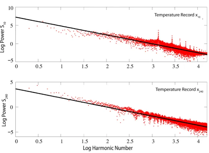
Of particular interest is the comparison of power spectra obtained from the 10 cm and 240 cm temperature sensors. A double-log plot of S10, shown in the upper panel ofFigure 5, reveals a striking pattern of discrete
peaks superposed over a quasi-continuum of harmonics over the range 0≤ ≤j 16, 000. The only other statisti- cally significant peak occurs at j=4 (not shown), corresponding to the annual period Ty
2
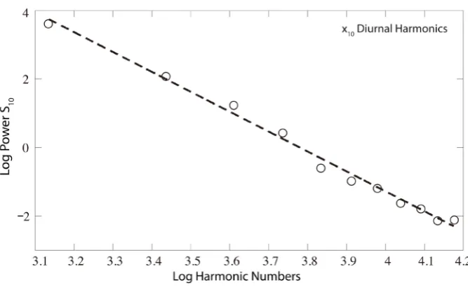
. A double-log plot of S240 in the lower panel shows the quasi-continuum of harmonics, but no evidence of discrete peaks. The
sequence of discrete peaks, shown separately as a double-log plot in Figure 6, corresponds precisely to the har- monic series3 T24 h
( )
n =24 n(
n=1, 2,)
of the diurnal period Td ≡1 d=24 h. All three double-log plotsreveal a power-law dependence S
( )
ν ∝ν−β on frequency ν over the observed range. Regression analysis leads to ML exponents(24 h)
10 5.82 0.55
β = ± (13)
for the diurnal harmonic spectrum S10(24 h) (Figure 6) and
240 1.83 0.068
β = ± (14)
2The peak at
y
T theoretically occurs at j=3.74. However, harmonic numbers must be integers.
Figure 4. Components at the fundamental frequency ω=2πTy in the Fourier analysis of temperature time series (a) y10; (b) y40; (c) y80; (d) y160; (e) y240. Phase shifts and amplitudes relative to y10 allow determination of the diffusivity D and agree with results of a
one-dimensional (1D) diffusion model.
Figure 5. Double-log plots of power spectra (red points) S10
( )
j (top panel) and S240( )
j (bottom panel) superposed by ML lines of regression (solid black). Both plots manifest a quasi-continuum of Brownian noise. S10( )
j also reveals a discrete series of diurnal harmo-nics jd.
for the quasi-continuous spectrum S240 (Figure 5). Exponent (14) is nearly the same for S10 upon removal of
the diurnal harmonic content.
Further elucidation of the spectral content of S240 is obtained by examining the power spectra of the 24-hour
averaged detrended series A24 hy240 and the 365-day moving average of the detrended series MA365 dy240 as
shown in Figure 7. The oscillatory structure seen in the spectrum of A24 hy240 does not signify multiple peri-
[image:6.595.148.482.83.259.2] [image:6.595.145.483.324.571.2]757
Figure 6. Double-log plot of S10
( )
jd (open circles) for the diurnal harmonics jd, super- [image:7.595.147.481.82.289.2]posed by ML line of regression (dashed).
Figure 7. Double-log plots of A24 hS240
( )
j (black dots) and MA365 dS240( )
j (red dots) with ML line of regression (dashed black).frequencies close to where ideally (i.e. in absence of noise) the Fourier transform of a pure sinusoid of period
y
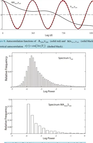
T vanishes, and the log approaches −∞. This interpretation is confirmed by the autocorrelation function (red trace) of A24 hy240 in Figure 8, which is fit exactly by the theoretical autocorrelation function
( )
cos 2π(
y)
r τ = τ T (dashed black trace). Upon removal of seasonal variability in the series MA365 dy240, the
sequences of cusps vanishes from the power spectrum inFigure 7(red dots), which is then fit very closely by a ML line of regression leading to power law exponent
(MA365 d)
240 1.996 0.008
β = ± (15)
characteristic of 1D Brownian diffusion. The periodicity at Ty largely vanishes from the autocorrelation in
Figure 8 (solid black trace), which then likewise (in accord with the Wiener-Khintchine theorem) manifests a long-range decay characteristic of a Brownian process.
Consider next the statistical distribution of the power spectral amplitudes—or a function of such ampli- tudes—which is useful in revealing empirically the probability density function (pdf) of a stochastic process. The objective of such an examination is to arrive at a recognizable form of pdf. InFigure 9 are shown histograms of logS240 (upper panel) and log MA
(
365 dS240)
(lower panel). In appearance the histogram of logS240 strong- [image:7.595.145.481.325.487.2]Figure 8. Autocorrelation functions of A24 hy240 (solid red) and MA365 dy240 (solid black);
theoretical autocorrelation r
( )
τ =cos 2(
πτ Ty)
(dashed black).Figure 9. Upper Panel: histogram of logS240 conforms to a hyperbolic distri-
bution. Lower Panel: histogram of log MA
(
365 dS240)
conforms to an expo- nential distribution. Elements of both histograms are partitioned among 100classes covering a harmonic range
(
214≥ ≥j 1)
.in fragmentation processes [15] [16], as well as stochastic processes involving diffusion of matter, energy or the movement of stock prices [17]. The pdf takes the general form [18]
(
)
1(
) (
)
2 2(
)(
)
; , , , exp 2
f xφ γ δ µ ∝ − φ γ+ x−µ +δ − φ γ− x−µ
(16)
759
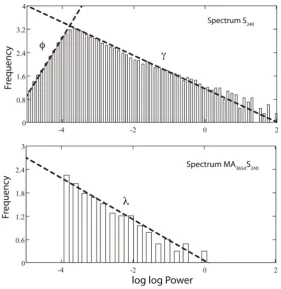
and δ >0 is a scaling parameter. The upper panel of Figure 10shows a histogram of log logS240, which re-
veals the hyperbolic form of the exponent in Equation (16) with visually fit asymptotic parameters φ=2.0, 0.57
γ = . The histogram of log MA
(
365 dS240)
in the lower panel ofFigure 9 strongly resembles an exponen-tial pdf whose general form is
( )
; exp(
)
f xλ ∝ −λx . (17)
Correspondingly, a plot of log log MA
(
365 dS240)
in the lower panel of Figure 10 reveals the linear form ofthe exponent in Equation (17) with visually fit parameter λ =0.53.
Although further investigation of the dynamical origin of these distributions is in progress, for the present purposes it suffices that spectral analysis and autocorrelation have revealed all statistically significant periodici- ties in the temperature time series.
5. Dynamics of Solar Energy Diffusion
A 1D diffusion model for temperature T x t
( )
, , based on the heat-flux equation [19]( )
2( )
2
, ,
T x t T x t
D
t x
∂ ∂
=
∂ ∂ , (18)
allows adequate prediction of time series x240 from the non-stochastic component of x10. The diffusivity
T
D=κ ρc (19)
depends on ground thermal conductivity κT, mass density ρ, and specific heat capacity c. The positive
di-rection of flow (x axis) is into the ground with origin at the surface. Solving Equation (18) for experimental conditions of this paper leads to
( )
( )
20
, 2 e cos d
2 x
D
T x t T t x
D
ω ω
ω ω ω
∞ −
= −
∫
(20)in terms of a theoretically known or empirically determined function T
( )
ω of angular frequency ω >0. When initial amplitudes{ }
θn and phases{ }
φn are known for a discrete set of fundamental frequencies{ }
ωn ,substitution of
( )
(
)
e nn n
n
i
T ω =
∑
θ δ ω ω− φ into (20) leads to the general form( )
20
, e cos
2
nx
n D
n n n
n
T x t t x
D
ω ω
θ θ − ω φ
= + − +
∑
, (21)which reduces to
( )
21 1
, e cos
2 x
D
T x t t x
D
ω ω
θ − ω φ
= − +
(22)
in the case of a detrended time series of single fundamental ω 2πTy 7.1726 10 4 h 1
− −
= = × .
Equation (22) permits estimation of the diffusivity D by two independent methods: 1) phase shift between corresponding maxima at times
(
t t1, 2)
of two temperature records of known depths(
x x1, 2)
2 2 1 p 2 1 1 4π y x x D T t t − = −
, (23)
and 2) amplitude attenuation of the peak temperature Tmax recorded at two known depths
( )
( )
2
2 1
a
max 1 max 2
π
log log
y
x x
D
T T x T x
−
=
−
. (24)
Figure 10. Upper Panel: histogram of log logS240 with visual fit to hyperbolic
asymptotes yielding slope parameters φ=2.0 , γ =0.57 . Lower Panel:
histogram of log log MA
(
365 dS240)
with visually fit line of regression yieldingslope parameter λ=0.53.
(
)
(
)
7 2 1p a 2 4.86 0.49 10 m s
D= D +D = ± × − ⋅ − . (25)
Given the value D in (25) and the amplitudes and phases
( )
(
)
(
)
1 10 1
2 10 2
3 10 3
3 11.562 0.864
1095 0.900 0.5
0.09 94
2190 0.162 81
c
c
c
θ φ
θ φ
θ φ
= = =
= = = −
= = =
(26)
from Fourier analysis of the mean-adjusted 3-year temperature record y10, including contributions at periods
y
T , Td, and 12Td (first diurnal harmonic), one can predict y240 from Equation (21), as shown in Figure 11.
The empirical (solid blue) and predicted (dashed black) time series agree very closely in amplitude and phase. The evidence supports the hypothesis that the observed subterranean temperature time series are the result of predominantly one-dimensional solar heat diffusion and that only this solar energy diffusion contributes to the trendline of MA365 dx240.
6. Conclusions
761
Figure 11. Comparison of detrended temperature series (red) y10 and truncated Fourier series
(solid black) y10( )3
( )
t +y10(1095)( )
t at fundamental periods Ty and Td. Comparison of detrend-ed temperature series (blue) y240 and solution (dashed black) T
(
240,t)
to the diffusionEquation (18) with boundary conditions based on y10.
transformations eliminating diurnal and seasonal variability, was found to be more than ten times the back- ground rate of global warming. This finding is consistent with surface temperatures recorded in central New York City, the second largest city in North America by population. There is no reason to think that these find- ings may be atypical for cities in industrialized countries. Given recent occurrences of extreme heat waves in the US and Europe, a precautionary conclusion, substantiated by climate modeling, is that, left unmitigated, the high rate of urban temperature rise relative to global warming will lead to more frequent and intense urban heat stress [20] [21].
Spectral analysis of the subterranean temperature time series at different depths revealed two distinct power laws suggestive of self-affine fractal behavior over the observed frequency range [22]. The exponent ~2 of the quasi-continuum spectrum is essentially independent of depth and corresponds to fractal Brownian noise (FBN) [23]. In general, FBN with ~ 3>βFBN >1 is more predictable than white noise (WN) for which βWN ~ 0,
such as observed in decay of radioactive nuclei [24]. For βFBN >2, the future trend follows the past trend,
whereas it reverses for βFBN <2. Brownian motion with βFBN =2 lies at the threshold between persistence
and anti-persistence because increments are uncorrelated.
The diurnal harmonic spectrum in the shallow subsurface temperature record can be shown [12] to arise from a non-sinusoidal heat flux due to unequal durations of daylight and darkness and the difference in rates of day- time heat absorption and nocturnal cooling. The large power-law exponent ~5.8 characterizes a relatively smooth function with behavior predictable by linear extrapolation. The development of an empirical model that accurately reproduces the diurnal power spectrum for purposes of understanding surface energy fluxes is in progress and will be reported when completed.
Acknowledgements
The author thanks Drs Jon Gourley and Christoph Geiss for several helpful conversations and the staff who maintain the Trinity College Weather Station and Temperature Well. Students who participated at short intervals in the project include Sarthak Khanal, Matthew Cohen, and Robert Tella.
References
[1] Tollefson, J. (2011) Nature News. http://dx.doi.org/10.1038/news.2011.607
[2] Cook, J., et al. (2013) Environmental Research Letters, 8, Article ID: 024024.
http://dx.doi.org/10.1088/1748-9326/8/2/024024
[9] Stone Jr., B. (2007) International Journal of Climatology, 27, 1801-1807. http://dx.doi.org/10.1002/joc.1555
[10] Union of Concerned Scientists (2006) Climate Change in the US Northeast. UCS Publications, Cambridge, MA, 10.
[11] Committee on America’s Climate Choices (2011) America’s Climate Choices. National Academy Press, Washington DC, 15.
[12] Silverman, M.P. (2014) A Certain Uncertainty: Nature’s Random Ways. Cambridge University Press (to be published), Cambridge.
[13] NYC Temperature Data. http://weather-warehouse.com/
[14] Shannon, C. (1949) Proceedings of the IRE, 37, 10-21. http://dx.doi.org/10.1109/JRPROC.1949.232969
[15] Silverman, M.P., Strange, W., Bower, J. and Ikejimba, L. (2012) Physica Scripta, 85, Article ID: 065403.
http://dx.doi.org/10.1088/0031-8949/85/06/065403
[16] Fieller, N.R.J., Flenley, E.C. and Olbricht, W. (1992) Applied Statistics, 41, 127-146.
http://dx.doi.org/10.2307/2347623
[17] Bibby, B.M. and Sorensen, M. (1997) Finance and Stochastics, 1, 25-41. http://dx.doi.org/10.1007/s007800050015
[18] Barndorff-Nielsen, O. (1977) Proceedings of the Royal Society of London. Series A, 353, 401-419.
http://dx.doi.org/10.1098/rspa.1977.0041
[19] Evett, S.R., et al. (2012) Advances in Water Resources, 50, 41-54. http://dx.doi.org/10.1016/j.advwatres.2012.04.012
[20] Wu, J., et al. (2014) Environmental Health Perspectives, 122, 10-16. http://dx.doi.org/10.1289/ehp.1306670
[21] Meehl, G. and Tebaldi, C. (2004) Science, 305, 994-997. http://dx.doi.org/10.1126/science.1098704
[22] Turcotte, D.L. (1997) Fractals and Chaos in Geology and Geophysics. Cambridge University Press, Cambridge, 148- 149. http://dx.doi.org/10.1017/CBO9781139174695
[23] Hergarten, S. (2002) Self-Organized Criticality in Earth Systems. Springer, Heidelberg, 48-66.
http://dx.doi.org/10.1007/978-3-662-04390-5
[24] Silverman, M.P. and Strange, W. (2009) Europhysics Letters, 87, Article ID: 32001.
currently publishing more than 200 open access, online, peer-reviewed journals covering a wide range of academic disciplines. SCIRP serves the worldwide academic communities and contributes to the progress and application of science with its publication.
Other selected journals from SCIRP are listed as below. Submit your manuscript to us via either