Representative Time Use Data and Calibration of the American Time Use Studies 1965 1999

Munich Personal RePEc Archive

Representative Time Use Data and

Calibration of the American Time Use

Studies 1965-1999

Merz, Joachim and Stolze, Henning

Forschungsinstitut Freie Berufe (FFB)

January 2006

Online at

https://mpra.ub.uni-muenchen.de/5856/

FFB

Freie Berufe

Fakultät II - Wirtschaft und Gesellschaft

Postanschrift:

Forschungsinstitut Freie Berufe Postfach 2440

21314 Lüneburg

[email protected] http://ffb.uni-lueneburg.de Tel: +49 4131 677-2051 Fax: +49 4131 677-2059

Universität

L Ü N E B U R G

Representative Time Use Data and Calibration of

the American Time Use Studies 1965-1999

Joachim Merz and Henning Stolze

Representative Time Use Data and

Calibration of the American Time Use

Studies 1965-1999

Joachim Merz und Henning Stolze

FFB Discussion Paper No. 54

January 2006

ISSN 0942-2595

Yale Program on Non- market Accounts: A Project on Assessing Time Use Survey Datasets

Research Institute on Professions (FFB), Department of Ec onomics and Social Sciences,

University of Lüneburg, Germany

________________________

Representative Time Use Data and

Calibration of the American Time Use Studies 1965 - 1999

Yale Program on Non- market Accounts: A Project on Assessing Time Use Survey Datasets

Joachim Merz und Henning Stolze

FFB Discussion Paper No. 53, December 2005, ISSN 0942-2595

Abstract

Valid and reliable individual time use data in connection with an appriate set of socio -economic background variables are essential elements of an empirical foundation and evaluation of existing time use theories and for the search of new empirical-based hypotheses about individual behavior. Within the Yale project of Assessing American Heritage Time Use Studies (1965, 1975, 19895, 1992-94 and 1998/99), supported by the Glaser Foundation, and working with these time use studies, it is necessary to be sure about comparable representative data. As it will become evident, there is a serious bias in all of these files concerning demographic characteristics, characteristics which are important for substantive time use research analyses.

Our study and new calibration solution will circumvent these biases by delivering a comprehensive demographic adjustment for all incorporated U.S. time use surveys, which is theoretically funded (here by information theory and the minimum information loss principle with its ADJUST program package), is consistent by a simultaneous weighting including hierarchical data, considers substantial requirements for time use research analyses and is similar and thus comparable in the demographic adjustment characteristics for all U.S. time use files to support substantial analyses and allows to disentangle demographic vs. time use behavioral changes and developments.

J EL: J22, J29, J11, Z0

Keywords: time use, calibration (adjustment re-weighting) of microdata, information theory, minimum information loss principle, American Heritage Time Use Studies, ADJUST program package

Zusammenfassung

Valide und zuverlässige individulle Zeitverwendungsdaten zusammen mit geeigneten sozio-ökonomischen Hintergrundvariablen sind essentiell für eine empirische Fundierung und Evaluierung bestehender Zeitverwendungs-theorien and für die Suche nach neuen empirisch fundierten Hypothesen über individuelles Handeln. Innerhalb des Yale Projektes ‘Assessing American Heritage Time Use Studies’ (1965, 1975, 19895, 1992-94 and 1998/99), das von der Glaser Foundation unterstützt wird, und der Arbeit mit diesen Zeitbudgetdaten ist es notwendig, sich auf die Repräsentativität mit vergleichbarer demographischer Struktur verlassen zu können. Wie ersichtlich wird, gibt es deutliche Abweichungen bei der Repräsentativität demographiacher Charakteristika in allen US Zeitverwendungs-studien, und zwar hinsichtlich demographischer Charakteristika, die bedeutend für die inhaltliche Analyse der Zeitverwendung sind.

Unsere Studie und die neue Hochrechnungslösung überwindet diese Verzerrungen mit einer demographischen Hochrechnung, die vergleichbar für alle US Files ist, theoretisch fundiert ist (hier durch die Informationstheorie und dem Minimum Information Loss Prinzip mit dem ADJUST Programmpaket), konsistent durch eine simultane Gewichtung ist, die hierarchische Daten beinhaltet, substantielle Anforderungen der Zeitverwendungsforschung unterstützt und es erlaubt, demographische Veränderungen von Verhaltensänderungen zu trennen.

J EL: J22, J29, J11, Z0

ii/120 Merz, Stolze: Calibration of American Time Use Studies 1965 - 1999

Contents

List of Tables

iv

List of Figures

v

Acknowledgements

vi

Executive Summary

vii

I

Introduction

1

II

The Adjustment/ Calibration of Microdata – Theory, Methods and ADJUST

software

3

The adjustment problem

4

Alternative adjustment procedures

4

The adjustment of microdata by the minimum information loss (MIL) principle

6

Absolute and relative adjustment factors

9

Multiple usages of re-weighting a sample

9

ADJUST software package

10

III

The Calibration of Time Diary Data – Particularities of Time Diary

Adjustments

10

Sample size considerations

11

Example: The German Time-Budget Study

12

IV

Choosing a Calibration Framework for Time Use Analyses

13

Dimensions of a calibration framework

13

Labor supply of women within the household context – The microeconomic

approach

14

Multiple market and non-market time use activities – socioeconomic analyses

16

Policy impacts of the tax and transfer system – Time allocation effects in the formal

and informal economy by microsimulation modeling

16

V

Adjusting Five American Time Use Studies

17

Heritage American time use data assessment and studies under investigation

17

Time use theory based and standardized calibration for all heritage files

18

Aggregate characteristics for the heritage files

20

Realization of the adjustment/calibration for all heritage files

26

Calibration results and experiences

31

VI

Disentangling demographic and behavioural changes – Re-calibration of the

US heritage files 1975-1999

35

Re-calibration results and experiences

35

VII Recommendations and Conclusions

37

References

39

Appendix A:

Adjustment Logfile 1965

45

Appendix B:

Adjustment Logfile 1975

50

Appendix C:

Adjustment Logfile 1985

55

Appendix D:

Adjustment Logfile 1985c

60

Appendix E:

Adjustment Logfile 1992-94

64

Appendix F:

Adjustment Logfile 1998/99

69

Appendix G:

Files containing new weights

74

Appendix DB:

Adjustment Logfile 1975-65

75

iv/120 Merz, Stolze: Calibration of American Time Use Studies 1965 - 1999

Appendix DD:

Adjustment Logfile 1985c-65

85

Appendix DE:

Adjustment Logfile 1992-94-65

90

Appendix DF:

Adjustment Logfile 1998/99-65

95

Appendix DG:

Files containing new weights -65

100

List of Tables

Table 1

Calibration procedures in different microsimulation models

5

Table 2

American time use studies under investigation

19

Table 3

Public holidays according to the U.S. code for the years of the heritage files

22

Table 4

Aggregates for the different heritage files

23

Table 5

Adjustment variables of the heritage files used to build the adjustment

microdata-matrix (S)

24

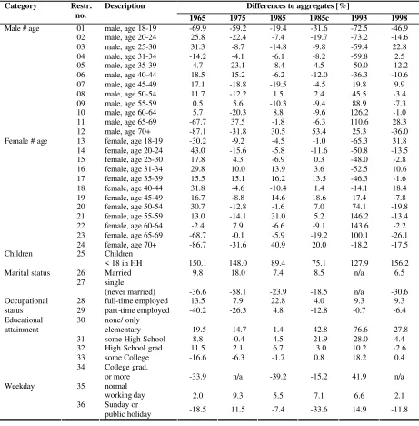
Table 6

Differences to the aggregates before the calibration

27

Table 6c Differences to the aggregates 1965 before the calibration

37

List of Figures

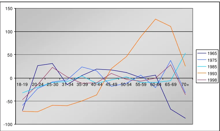
Figure 1

Representation of American Heritage Time Use Files 1965 – 1998/99 -

Over- and underrepresentation compared to desired totals in %: Males by

age classes

28

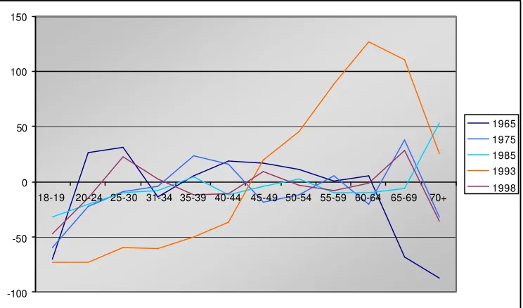
Figure 2

Representation of American Heritage Time Use Files 1965 – 1998/99 -

Over- and underrepresentation compared to desired totals in %: Females

by age classes

29

Figure 3

Representation of American Heritage Time Use Files 1965 – 1998/99 -

Over- and underrepresentation compared to desired totals in %: Family

status

29

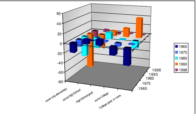
Figure 4

Representation of American Heritage Time Use Files 1965 – 1998/99 -

Over- and underrepresentation compared to desired totals in %:

Educational attainment

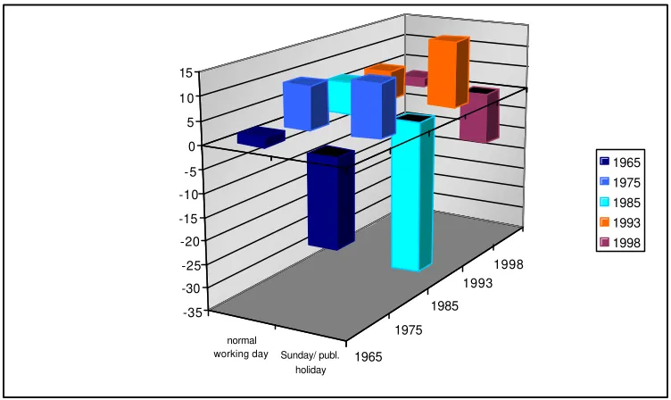
Figure 5

Representation of American Heritage Time Use Files 1965 – 1998/99 -

Over- and underrepresentation compared to desired totals in %:

Representation of days of the week

31

Figure 6

Frequency distributions of the old and new weight of the 1965 American

Time Use Survey

32

Figure 7

Frequency distributions of the old and new weight of the 1975 American

Time Use Survey

32

Figure 8

Frequency distributions of the old and new weight of the 1985 American

Time Use Survey

33

Figure 9

Frequency distributions of the old and new weight of the 1985c American

Time Use Survey

33

Figure 10

Frequency distributions of the old and new weight of the 1992-94

American Time Use Survey

34

Figure 11

Frequency distributions of the old and new weight of the 1998-99

American Time Use Survey

34

Acknowledgements

This paper is a part of the project

Assessing Time Use Survey Datasets

supported by Yale

University with Dr. Andrew S. Harvey (Project Head), Time Use Research Program (TURP), at

St. Mary’s University, Halifax, NS, Canada; Dr. Ignace Glorieux, Tempus Omnia Revelat

(TOR), Faculty of Economic, Social and Political Sciences, Vrije Universiteit Brussel, Brussels,

Belgium; Dr. Joachim Merz, Research Network on Time Use (RNTU), Research Institute on

Professions (FFB), Department of Economics and Social Sciences, Unive rsity of Lüneburg,

Lüneburg, Germany; and Klas Rydenstam, Statistics Sweden.

Many thanks to Diane Herz (Bureau of Labor Statsistics, USA), and her colleagues for providing

the CPS information and all the support. We also wish to thank participants of the IATUR 2005

vi/120 Merz, Stolze: Calibration of American Time Use Studies 1965 - 1999

Executive Summary

Valid and reliable individual time use data, in connection with a proper set of socio

-economicbackground variables, are essential elements for the empirical foundation and

evaluation of existing theories, and the search for new empirical-based hypotheses about

individual behavior in the household context. Several potentially useful time use heritage

datasets have been identified for use in developing an historical series of non-market accounts. In

order to evaluate the series of heritage U.S. time use surveys (1965, 1975, 1985, 1992-94,

1998-99), it is necessary to be certain about representativeness of the data.

As our analyses will show, the five U.S. heritage files - based on the given survey weights - are

seriously biased according to important demographic totals which in addition are of strategic

importance for substantial time use analyses. This study reports a solution that circumvents

several shortcomings in delivering a comprehensive demographic adjustment to all incorporated

U.S. heritage time use surveys. This adjustment is theoretically founded on information theory,

consistent by a simultaneous weighting including hierarchical data like personal and

family/household data, ensures desired positive weights, considers substantial requirements for

time use research analyses, and is similar in the demographic adjustment characteristics for all

heritage files thus facilitating substantial analyses and disentanglement of demographic vs. time

use behavior changes and develo pments.

First part of this study – calibration for representative US time use heritage files

The first part of the study describes the calibration/adjustment procedure and its theoretical

background, discusses and presents the demographic frame used for all five US heritage files,

computes, delivers and describes five sets of new sample weights which guarantee the respective

demographic totals.

Second part of this study – calibration io disentangle behavior from demographic changes

The second part provides four sets of alternative sample weights which allows to disentangle

changes in time use behaviour from changes in the population structure. These alternative sample

actual survey compared to the 1965 population, compute , deliver and describe the new

alternative weights for all remaining four time use surveys.

Our study has clearly shown that if using the Heritage US time use data with the given

old calibration, the bias in the results of substantial analyses would be not negligible. This holds

true in particular for characteristics with an obviously strong connection to individual time use

behavior (like the respondent’s age or the number of children); the results would be heavily

under- or overrepresented respectively. In general, relying on uncalibrated data would inevitably

lead to questionable conclusions.

With the available new five sets of consistent and similar structured weighting factors, it

is possible, in particular, to follow up American time use behavior for about 40 years based on a

reliable and valid demographic background delivering representative data for substantial time

use analyses.

In addition, the re-calibrated younger US heritage files all with the 1965 population

structure now are available for substantive analyses in disentangling demographic from time use

behavioral changes.

Based on our calibration experience we recommend above all that

•

For any new time use survey, the calibration procedure and the single substantial

definitions of the adjustment characteristics with their totals have to be documented

carefully.

•

A new adjustment of a new ATUS file should be as close as possible to the used

adjustment characteristics of the older ones to ensure a common demographic

background with no biased results if using a different approach.

•

Since the software Adjust can be operated easily on every desktop-computer, sensitivity

analyses with different totals resulting in different weighting sets will help further to

disentangle demographic effects from behavioural effects.

Without a proper calibration of the US heritage time use files, a necessary and important

prerequisite for any further substantive analyses would be missing and substantive results not

Merz and Stolze: Representative Time Use Data and Calibration of the American Time Use Studies 1965-1999 1/120

I

INTRODUCTION

Valid and reliable individual time use data, in connection with a proper set of

socio-economicbackground variables, are essential elements for the empirical foundation and

evaluation of existing the ories, and the search for new empirical-based hypotheses about

individual behavior in the household context. Several potentially useful time use heritage

datasets have been identified for use in developing an historical series of non- market accounts. In

order to evaluate the series of heritage U.S. time use surveys (1965, 1975, 1985, 1992-94,

1998-99), it is necessary to be certain about representativeness of the data.

As our analyses will show, the five U.S. heritage files - based on the given survey weights - are

seriously biased according to important demographic totals which in addition are of strategic

importance for substantial time use analyses. This study reports a solution that circumvents

several shortcomings in delivering a comprehensive demographic adjustment to all incorporated

U.S. heritage time use surveys. This adjustment is theoretically founded on information theory,

consistent by a simultaneous weighting including hierarchical data like personal and

family/household data, ensures desired positive weights, considers substantial requirements for

time use research analyses, and is similar in the demographic adjustment characteristics for all

heritage files thus facilitating substantial analyses and disentanglement of demographic vs. time

use behavior changes and develo pments.

First part of this study

The first part of the study describes the calibration/adjustment procedure and its theoretical

background, discusses and presents the demographic frame used for all five US heritage files,

computes, delivers and describes five sets of new sample weights which guarantee the respective

demographic totals.

Re-weighting of the heritage time use data was necessary for several reasons. First, due to

the lack of documentation, it was not possible to get sufficient information about the calibration

according to the weighting procedure and the totals (margins) to be achieved. Therefore, a

theoretically founded and transparent adjustment is needed.

Second, as far as we know, not all of the weightings of the different heritage files use an

(weighting, calibration), which simultaneously fulfills hierarchical information (e.g. Household

and personal information), is not assured. It is necessary to remedy this.

Third, the demographic information used in the adjustments should consider substantial

requirements of time use research analyses.

Fourth, a similar demographic adjustment scheme for all single heritage files was not

available. Such a scheme is desirable for concentrating on substantial behavioral changes

independently of further demographic developments.

To achieve representative results and to check whether five U.S. time use surveys (1965,

1975, 1985, 1992-94, 1998-99) fulfill the necessary requirements, we apply a consistent solution

of the microdata adjustment (calibration) problem: a proper (re-)weighting of microdata to fit

aggregate control data via the min imum information loss principle based on information theory

using the Adjust software.

Second part of this study

The second part provides four sets of alternative sample weights which allows to disentangle

changes in time use behaviour from changes in the population structure. These alternative sample

weights use the demographic totals from the oldest survey 1965 as the new demographic totals

for the younger files within the new calibrations. We describe the population changes of the

actual surve y compared to the 1965 population, compute , deliver and describe the new

alternative weights for all remaining four time use surveys.

This paper is divided as follows: In the first part, after briefly describing the

methodological background of our adjustment procedure based on the information theory,

including a survey of used alternative calibration procedures (chapter 2), we discuss

particularities of time use diary adjustments, and show a solution within the actual German Time

Use Survey (chapter 3). In chapter 4, a calibration framework for time use analyses is chosen,

sketching the microeconomic labour supply of women within the household context, household

production/time allocation, mult iple market and non-market analyses, as well as policy impacts

of tax and transfer systems, and alternatives. Chapter 5 provides the results of the new

Merz and Stolze: Representative Time Use Data and Calibration of the American Time Use Studies 1965-1999 3/120

The second part of this study is about disentangling demographic changes from changes

in time use behavior by re-calibrating the US heritage files 1975 – 1999 based on the

demographic structure of 1965 (chapter 6).

Chapter 7 presents study conclusions and gives some recommend ations.

II

THE ADJUSTMENT/CALIBRATION OF MICRODATA – THEORY, METHODS

AND ADJUST SOFTWARE

To adjust/calibrate microdata is to fit microdata to prescribed and known aggregate totals

(with synonyms as control data, restrictions, margins, population totals). For each microunit of a

(sample) microdata file, a suitable weight is searched so that the weighted sum of all microunit

cha racteristics will achieve their externally given aggregates.

A microdata matrix S consists of microunits such as persons, families, households, or

firms which are described by various characteristics. If, for example, these microunits are

per-sons, they would be described by age, gender, employment, or other characteristics which

correlate with the current topic under investigation.

The known population characteristics derived from, for example, a census, restrict the

microdata to their desired total values. Aggregate statistics will deliver single restrictions, or a set

of constraints, which could be given as a multidimensional cross tabulation. In general, the

restrictions may be given by official aggregate statistics, by other samples, or by other models.

Aggregate sample information, for example, may be given by a population census or a more

frequent microcensus with demographic variables, labour force participation information, etc. In

our application here, the American Current Population Survey (CPS) an ongoing monthly

household survey to provide demographic and labor force information is delivering the totals to

be achieved. Since the CPS is adjusted to the Census the calibration will fit the Census data.

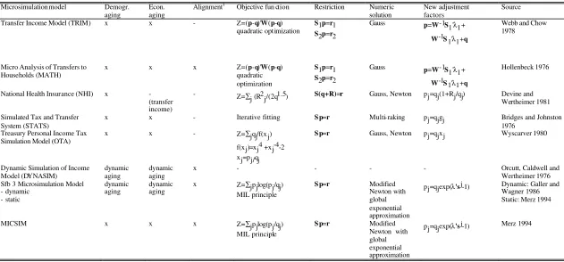
The calibration of microdata is a common method in microsimulation models, where it is

used not only to extrapolate a data set (static aging), but also for sensitivity analyses using

alternative totals. Table 1 presents an overview of a selection of calibration procedures used in

microsimulation models.

As Table 1 shows, there are different calibration procedures with different objective

functions, such as the CALMAR approach used in the SAS framework. However, most of them

and new weights) to be min imized resulting in possible zero or negative weighting factors. Since

non positive weights will further exclude microunits, only a procedure which provides positive

weights, such as the approach used in this paper, is appropriate.

The adjustment problem

In general, the adjustment problem is to find an n-vector p of adjustment factors

opti-mizing an objective function Z(p,q) - a function evaluating the distance between the new

adjustment factors p to be computed and the available factors q - satisfying the m re strictions

Sp=r:

(1)

Z(

p

,

q

) = min! s.t.

Sp

₌

r

.

This adjustment problem is a simultaneous one where, for even a large number of

cha racteristics (n), only a single weighting factor has to be computed for each microunit which

after summing up, fulfils consistently all m hierarchical microdata totals (e.g. household, family

and personal information) simultaneously.

The objective function minimizes the distance between new adjustment factors p and the

given factors q in order to capture already available information and corrections due to

non-response, sampling errors, etc. If such corrections are not given in advance (or as a simple

microunit independent sampling ratio), q

would be equal for each microunit j (j=1,...,n). In the

case of demographic features in the sample information matrix S (and the restrictions), a single,

absolute adjustment factor for a sample micro unit j represents p

total population microunits.

Alternative adjustment procedures

There are various procedures and functional forms in quantitative economics where an objective

function Z(

p

,

q

) weight the distance of two (adjustment) factors. In general, procedures with

quadratic (unweighted or weighted) and other objective functions (linear or nonlinear) are

conceivable. Within the Microsimulation context and its static aging (re-weighting by more

Merz and Stolze: Representative Time Use Data and Calibration of the American Time Use Studies 1965-1999 5/120

Table 1 Calibration procedures in different microsimulation models

Microsimulation model Demogr. aging

Econ. aging

Alignment1 _{Objective fun ction Restriction Numeric}

solution

New adjustment factors

Source

Transfer Income Model (TRIM) x x - Z=(p-q)'W(p-q) quadratic optimization

S₁p=r₁ S₂p=r₂

Gauss _p=W-1_S 1'λ1+

W-1S_1'λ₁₊q

Webb and Chow 1978

Micro Analysis of Transfers to

Households (MATH) x x x Z=(

p-q)'W(p-q) quadratic optimization

S₁p=r₁ S₂p=r₂

Gauss _p=W-1_S 1'λ1+ W-1S_1'λ₁₊q

Hollenbeck 1976

National Health Insurance (NHI) x - (transfer income)

- _Z=∑

j (R2j/(2q1.5) S(q+R)=r Gauss, Newton pj=qj(1+Rj/qj) Devine and _{Wertheimer 1981}

Simulated Tax and Transfer System (STATS)

x x - Iterative fitting S p=r Multi-raking _pj=qjgj Bridges and Johnston 1976

Treasury Personal Income Tax

Simulation Model (OTA) x x - Z=∑jqj/f(xj) f(xj)=xj4 +xj-4-2 xj=pj/qj

S p=r Gauss, Newton _pj=qjxj Wyscarver 1980

Dynamic Simulation of Income Model (DYNASIM)

dynamic aging

dynamic aging

x - - - - Orcutt, Caldwell and

Wertheimer 1976 Sfb 3 Microsimulation Model

- dynamic - static

dynamic

aging dynamic aging x Z=_{MIL principle} ∑jpjlog(pj/qj) S p=r Modified Newton with global exponential approximation

pj=qjexp(λ'sj-1) Dynamic: Galler and

Wagner 1986 Static: Merz 1994

MICSIM x x x Z=∑_{jpjlog(pj/qj)}

MIL principle

S p=r Modified Newton with global exponential approximation

A solution based on a quadratic and unweighted objective function is used, for example, by

Galler 1977 to determine a consistent adjustment procedure for the Integrated Microdata File

(IMDAF-69) of the SPES project and its successor, the Sonderforschungsbereich 3 (Sfb 3)

'Microanalytic Foundations of Social Policy' at the Universities of Frankfurt and Mannheim,

Germany. Hollenbeck 1976 proposed a quadratic weighted objective function for the

adjustment of the micromodels of Mathematica Policy Research, Inc. (MPR) and The Policy

Research Group, Inc. A constrained quadratic loss function is also used for instance by Stone

1976 and extended by Byron 1978 in an input/output context to estimate large social account

matrices. Different algorithms may solve the quadratic programming approach (e.g. by Frank

and Wolfe 1956, Hildreth 1957 or Houthakker 1960). These operations research procedures,

however, become relatively inconvenient for large adjustment problems, particularly those

with many microunits and many characteristics.

Oh and Scheuren 1980 took a multivariate raking ratio estimation in their 1973 exact match

study to fit several types of sample units (design, analysis and estimation units) (see their

bibliography on raking). The raking ratio estimation, reaching back to Deming and Stephan

1940, uses proportional factors in each iteration to fit the marginals of a multi-way table (see

also 'iterative proportional fitting' in Bishop and Fienberg 1975 and the log linear approach

within contingency tables in Mosteller 1968); this approach will be simular to our weighting

procedure based on the minimum information loss principle..

Another, relative simple, weighting approach is the well known Horvitz-Thompson estimator

as the inverse of the sampling ratio. This weighting approach is only well suited for real

random samples, but not sufficient for the utimate non-random survey at hand. For a further

treatment of different approaches, like algorithms connected with input/output tables, and

procedures see Wauschkuhn 1982 and Merz 1986, Chapt. 7.

The adjustment of microdata by the minimum information loss (MIL) principle

.As seen above, there are many attempts to weight a sample However, those

procedures may produce negative adjustment factors, or zero factors when restricted. But

non-positive adjustment factors cannot be interpreted meaningfully in applied work because

an adjustment factor has to represent a certain number of households or persons. Therefore,

strictly positive weights are required to keep all sample microunits for further analyses.

Another prerequisite is to take care of adequate weights according to personal and

Merz and Stolze: Representative Time Use Data and Calibration of the American Time Use Studies 1965-1999 7/120

weights, as often used in survey weighting, will not ensure the simultaneous fit to the

aggregate personal as well household data.

A solution procedure is described which ensures the positivity constraint by an

appropriate objective function as well as the simultaneous requirements via appropriate

handling a set of hierarchical restrictions. Our objective function is theoretically based on

information theory, which optimizes a logarithmic function according to the Minimum

Information Loss Principle. In recent years, information theory - well known in engineering

sciences - has found some applications in economics. Theil's 1967 'information inaccuracy' is

used, for instance, to judge the forecasting accuracy of econometric models (Merz, 1980).

Measuring income inequality by an approach based on information theory is another example

(Theil, 1972; Foster, 1983). More recently, minimum information was used to estimate

microeconomic allocation models (Theil, Finke and Flood, 1984; Finke and Theil, 1984).

Based on the probability distribution p

with

p

= (p

,...,p

)’, (p

>0),

∑

p

= 1,

(j = 1,...,n), the entropy or information content of

p

is defined as

(3a)

H(

p

) = H(p

,...,p

) =

∑

p

log(1/p

).

An extension of the entropy concept is the

information loss

(or gain) when a multinomial

distribution

q

= (q

,...,q

)' is substituted by a similar distribution

p

= (p

,...,p

)'

(3b)

I(

p

:

q

) =

∑

p

log(1/q

) -

∑

p

log(1/p

) =

∑

p

log(p

_/qj),

with

(p

,q

>0),

∑

p

=

∑

q

= 1, (j=1,...,n).

Within this concept, the information loss is evaluated as the expected information

before, weighted by p

, minus the expected information after substitution. For an axiomatic

derivation of the connected maximum entropy principle or principle of minimum

cross-entropy, see Shore and Johnson (1980), and Jaynes (1957) who first proposed entropy

maximization within engineering purposes.

The information theory based approach, as well as the approach with a quadratic

distance function, are specific cases of the generalized entropy class

(3c)

I

_α

(

p

,q) = [N

Σ

_j(pj

α

q1-

α

-q)] / [

α

(

α

-1)],

with uniformly distributed adjustment factors qj=q=1/n, and where N is the number of all

microunits in the population. The quadratic objective function is given for

α

=2 with

1 _{As to Atkinson, Gomulka and Sutherland 1988 p. 230 who refer to the MIL adjustment procedure by Merz}

I

(

p

,q) = 1/2

Σ

(p

- q)

_{divided by q. The information theory based approach is given for}

_α

=1. Since the derivative of 3c with respect to pj is Np

/ (

-1), the information based

approach can be interpreted as that measure with the largest value of

α

, where the first

derivative approximates minus infinity, and the weight approximates to zero (satisfying the

positivity constraint).

With reference to the above information theory concept, the adjustment problem

under the minimum information loss (MIL) principle

is to minimize the objective function

(4a)

Z(

p

,

q

) = min

{

∑

p

log(p

/q

)}

(4b)

s.t.

Sp

=

r

.

where

p

_j

= new adjustment factor for a microunit (e.g. household) j (j=l,...,n);

q

_j

= available

(known) adjustment factor for each micro unit j, n=number of micro units, with

S

_{(m,n) = [sij]}

sample information matrix (i=1,...,m; j=1,...,n),

r

_{(m) = [ri] vector of restrictions, m=number}

of restrictions. The MIL-objective function minimization subject to the simultaneous set of

possible hierarchical restrictions fulfills the two main requirements of positive weights and

simultaneous consideration of hierarchical data.

As a solution condition, it is necessary that a) the number of micro units in a random

sample is higher than the number of characteristics (n

≥

m), and b) the matrix

S

is row regular,

meaning that the distribution of the individual characteristics in a random sample is linear

independent (rank

S

=m). Generally, the usual condition a) will be fulfilled; condition b) can

be guaranteed by omitting one respective characteristic from an exhaustive polytomuous

distribution.

The Lagrangean is

(5)

L(

p

,

λ

) =

∑

p

(logp

- logq

) -

λ

'(

Sp

-

r

),

which yields a nonlinear equation system

(6)

∑

s

q

exp(

λ

'

s

- 1) = r

(i=1,...,m),

that has to be solved for the Lagrange multipliers

λ

_{k (k=1,...,m) iteratively.}

The new adjustment factors

with the solution

λ

are

(7)

p

= q

exp(

λ

'

s

- 1),

where

s

j are the respective characteristics of the microunit j.

Thus, the new adjustment factors can be calculated relatively simply: the single given

Merz and Stolze: Representative Time Use Data and Calibration of the American Time Use Studies 1965-1999 9/120

the respective microunit (e.g. household and personal) characteristics (

s

) and the Lagrange

multipliers. Therefore, it is possible to determine the new adjustment factors after calculating

λ

independent of all other microunits and thus also independent from the sample size. This is

important for practical work with mass (micro) data.

Absolute and relative adjustment factors

Usually the above adjustment factors

p

_j

and

q

_j

are not formulated as probabilities

respectively relative frequencies with 0<p

,q

<1,

∑

p

=

∑

q

= 1, but rather in absolute terms.

The absolute adjustment problem,

(8)

Z(

p

,

q

) = min

{

∑

p

log(p

/q

), s.t.

Sp

=

r

}.

yields the same solution (8) as in the relative case and is only different according to the

interpretation with p

= p

N, q

= q

N and r

= r

N (N = number of all microunits in the total

population).

In the absolute case, a sample weight p

(j=1,...,n) then represents the actual number

of microunits (say households if the weights correspond to this type of microunit) in the total

population. The restriction r

(i=1,...,m) is then the absolute number of microunits with

characteristic i (e.g. households with three persons and a self-employed household head) in

the total population. The sample information matrix

S

remains the same in both cases and

describes the microunits' characteristics in the sample.

If there are no specific weighting factors given in advance (free adjustment) and/or

the sample under consideration would be a (pure) random one with an overall sampling ratio

w = [sample size(n)/population size(N)] (like w=1/100 in a 1% microcensus case), then the

old weights would be equal for each microunit j: In the relative case q

= q = 1/n, and in the

absolute case q

= q

N = (1/n)N = N/n = 1/w as the inverse of the sampling ratio (w=n/N) (for

example q

= q = 100 in a 1% microcensus case) for all microunits j (j=1,...,n).

Multiple usages of re-weighting a sample

The calibration of microdata can be used not only to adjust a specific sample to its totals

•

Achieving representative results for a given sample and its population

- Descriptive microanalyses

- Micreoeconometrics: weighted estimation

•

Sensititivity analyses with alternative artificial totals and respective weightings

•

Extrapolating/forecasting samples for an actual demographic situation

•

Microsimulation context: static aging (forecasting by re-weighting), weighting of

simulation files

ADJUST software package

Our program package ADJUST fulfils the above requirements in an efficient manner for

unlimited sample sizes. ADJUST has been proven to be successful in many applications: for

the adjustment of the recent Time Budget Survey of the German Statistical Office and a

refined adjustment of the German Socio-Economic Panel; within the framework of a

microsimulation analysis of financial and distributional impacts of the German Pension

Reform; a consistent adjustment for the microsimulation analysis of time allocation impacts

in the formal and informal economy of the recent German tax reform. In addition, ADJUST

has been used in applications at the London School of Economics (LSE, UK), at the

Australian Bureau of Statistics (ABS) with the National Centre of Simulation, and Economic

Modelling (NATSEM) at the University of Canberra (Australia). ADJUST is available via

http://ffb.uni-lueneburg.de/adjust

.

III

THE CALIBRATION OF TIME DIARY DATA – PARTICULARITIES OF

TIME DIARY ADJUSTMENTS

To increase the representativeness of a sample, the calibration has to be based on

variables which have a substantial influence on time use behavior. To find appropriate

aggregates to support substantial time use analyses, we refer to socio-demographic

backgrounds of ind ividuals based on human capital and performance characteristics as well

as to socio-cultural backgrounds of the families and households. In addition, day specific

information with expected time use influences via workdays or weekends should be

integrated within the calibration procedure. Thus a simultaneous calibration approach, which

Merz and Stolze: Representative Time Use Data and Calibration of the American Time Use Studies 1965-1999 11/ 120

To improve the quality and representativeness of survey data, a set of new (re-)

weighting factors has to be computed. In the first step, weights have to be found for each

observation which adjust the biased sample selection resulting from unproportional quotas

(e.g. from oversampling of highly interesting but small demographic groups) or not fulfilled

quotas. The second step builds upon the weights found in the first free adjustment procedure.

Its aim is to create adjustment factors in such a way that the weighted sums of variables meet

externally given aggregate values.

Due to the non-randomness of the sample (e.g. quoted samples) and missing

observation units etc., the demographic structure of the time-budget survey might differ from

the actual population measured by another official statistic (e.g. a micro-census or population

survey file). By using new adjustment factors, the differences between the aggregated survey

data and the preferred aggregates should vanish. This is especially important when dealing

with variables which might correlate with the time use-behavior. More specific details on

how to choose appropriate characteristics are discussed in the following chapter.

In addition to the demographic structure variables, the distribution of time data itself

(e.g. days over the week or the season of the survey) may be biased and is likely to influence

the time use behavior. It is expected that one will observe different activities in the summer

than in the winter, and that time use patterns will vary between working days and Sundays.

Public holidays should be taken into account as well. Even with quoted samples it is difficult

to match these aggregate distributions. As a result, date and time information should be

considered in the adjustment as well.

Sample size considerations

Though a deeply disaggregated multidimensional set of adjustment characteristics is

desired,, however, the size of the sample often limits the structure of the aggregates in that

mostly one or two-dimensional aggregate distributions can be used. Combining

characteristics would often result in classes with very few, if any observations, therefore most

of the aggregates can only be computed separately. This means, for example, that the

weighted sum of 2-person-households and the weighted sum of blue-collar-workers will both

The selection of characteristics used in the adjustment procedure underlies two major

considerations. First, the number of characteristics influences the quality of the results. If too

many variables are chosen, then the algorithm may not find a numerical solution and the

range between lowest and highest adjustment factor will grow rapidly. Additio nally, some

categories without observations may occur, so the sample file cannot meet the aggregates in

these aspects. Second, the chosen characteristics should be correlated with the time use

behavior and should include the characteristics used in the sample.

Example: The German Time-Budget Study

Due to the non-randomness of the sample (caused by over sampling of certain

subgroups) and missing observation units, the demographic structure of the time-budget

survey differs from that of the German micro-census. As a result, a calibration to correct

these biases (using the ADJUST-software approach and the approach used in our study here)

has been applied to both German time budget studies in 1991/92 and 2001/02. The fo llowing

characteristics have been used for this task:

(a) For households:

•

States

•

Phase of the survey crossed with region (West-/ East-Germany) code

Social situation crossed with the region code

•

Size of the household crossed with region code

•

Size of the community crossed with region code

•

Household-type crossed with region code

•

Only for the adjustment of the episode data: Day of the week [Mon-Thu; Fri; Sat;

Sun]

(b) For persons:

•

States

•

Phase of the survey crossed with region (West-/ East-Germany) code

•

Social situation crossed with the region code

•

Size of the household crossed with region code

•

Size of the community crossed with region code

Merz and Stolze: Representative Time Use Data and Calibration of the American Time Use Studies 1965-1999 13/ 120

•

Only for the adjustment of structural data: occupational status crossed with region

code and with gender

•

Only for the adjustment of episode data: occupational status crossed with day of the

week and gender crossed with day of the week

With respect to information on the day of the week, the following calibration was

used: for each participant two days were observed so the adjustment factors for the episode

data project two days (8/7

normal workdays [Monday thru Thursday], 2/7

Fridays, 2/7

Saturdays and 2/7

Sundays adding up to 14/7

or 2 days).

IV

CHOOSING A CALIBRATION FRAMEWORK FOR TIME USE ANALYSES

There are two central dimensions of time use analyses: first is the time itself, which

can be spent in a multitude of market and non-market activities with an appropriate

measurement by main and secondary activities (endogenous variables). The second

dimension, which is at least as important as the first, encompasses the socioeconomic

background variables to explain ind ividual behavior (explanatory, exogenous variables).

Dimensions of a calibration framework

The aim is to find a calibration framework which allows valid demographic data to

analyze time use behavior based on different theoretical socioeconomic approaches. To find

such a calibration kernel, we briefly discuss the importance, necessity and application of time

use information in explaining behaviors for theoretically based empirical and integrated

economic and social research, as well as for a targeted economic and social policy.

As a basis, we sketch the economic framework of activity linked time dimensions: the

optimal allocation of goods and time with constrained goods and time resources. Within this

framework, the microeconomic allocation model, the optimal labor supply, and the household

production approach for a model of multiple market and non-market activities is of central

importance. Individual time use data, in connection with a proper set of background

variables, are essential for an empirical foundation and an evaluation of those theories (‘new

home econo mics’), as well as for the search of new empirical based hypotheses about

individual behavior in the household context.

1.

Labour supply of women within the household context – microeconomic analyses

2.

Household production/time allocation

3.

Multiple market and non-market time use activities – socioeconomic analyses

4.

Policy impacts of the tax and transfer system – time allocation effects in the formal

and informal economy by microsimulation modeling.

These examples and research areas will illustrate the need for and the spread of appropriate

background variables and demographic calibration requirements.

Labour supply of women within the household context – the microeconomic approach

Within the well known microeconomic allocation model, an individual/household is

maximizing his/her/its utility based on the amounts of goods. Facing a restricted income,

utility maximization under the money constraint yields an optimal allocation of goods in a

static or an intertemporal approach. Based on this microeconomic allocation model, the

individual’s paid working hours (labor supply) are incorporated in the preference

optimization model via leisure (full time minus leisure determines the working hours). Thus,

total time is divided into consumption time (leisure) and time for paid work to earn income.

Then, maximizing utility as a function of the market goods amounts and the consumption

time subject to full income (all expenditures plus wage weighted cons umption time equals

non-labor income and wage weighted total time) yields the optimal allocation equations for

the goods amounts as well for the working hours (labor supply).

Already within this classical approach socio-economic background variables are

necessary for

•

individual utility function dependent of the socioeconomic status

•

individual wage, including the potential wage of nonworkers, which has been

econometrically estimated by socioeconomic variables

•

non-labour income dependent of the socioeconomic status

hours of paid work.

Within the last decade, empirically based labour supply research based on advanced

econometric methods has proven the importance not only of time use itself in paid work, but

also the need for proper socioeconomic background variables with regard to the mentioned

four microeconomic dimensions.

Merz and Stolze: Representative Time Use Data and Calibration of the American Time Use Studies 1965-1999 15/ 120

family dependent labor force participation) is important. [Useful literature includes the survey

concerning labor supply by Killingsworth, 1983; concerning female labor supply by

Killingsworth and Heckmann, 1986; as well as recent issues in scientific journals (e.g.

Journa l of Labor Economics)].

In brief: personal as well household characteristics have to be valid for following this

strand of time use research.

Household production/time allocation

With the ‘new home economics’ since the Nobel prize winner Becker (1965),

Lancaster (1966), Muth (1966), and Ironmonger (1972), the above microeconomic approach

has been broadened by household production and the connected time allocation. The utility

function is now based on the basic commodities which are produced by the househo ld with

its input of non-market time and market goods. Such commodities can be defined broadly

(e.g. childcare, homework, and do-it-yourself work). Shadow prices can be assigned for the

basic commodities, which have no market price per se, via the dual approach. Dependent of

the household technology the shadow prices are dependent or independent of the household

production output amount.

Within this approach, the optimal allocation problem is solved in three steps:

•

Modeling the efficient household technolo gy (duality between production and cost

function)

•

Modeling and calculation of the shadow price (price of the basic commodities,

duality of cost function, and valued production)

•

Utility maximized allocation with regard to output (with shadow prices) or with

regard to input (with explicit functionalized market goods and the necessary time

for the production).

In all three steps, an empirical sound model needs the appropriate personal and household

socioeconomic background variables in addition to the income restriction and the empirically

Multiple market and non-market time use activities – socioeconomic analyses

To explain and estimate a proper household production of different commodities,

different time inputs and their dependencies to the socioeconomic background are necessary.

If this approach is expanded by multiple paid market activities (multiple labour supply) –

possibly including tax and transfer evading black work – then a full multiple market and

non-market time use activity model can be formulated which will overcome the traditional

one-sided focus on paid work alone.

The theoretical modeling approach allows for the formulation of the impacts of

changing model parameters (like the income and substitution effects of a price/ wage

change). However, only an empirically based estimation and explanation with proven

socioeconomic hypotheses will finally quantify these effects and decide, for example,

whether the income or the substitution effect will be dominant – an important result in

explaining the final labor supply.

To do this, detailed time use information on multiple activities are necessary, and

above that, and this has to be underlined, the right set of socioeconomic background variables

are essential for all of the needed theoretically based above model variables. This is important

for testing given models with a multitude of preferences and background, and for finding new

hypotheses of what the people do via and connected by and with its time individual

dimension in the household and their regional labor market and economic context.

Policy impacts of the tax and transfer system – time allocation effects on the formal and

informal economy by microsimulation modeling

Explaining behavior is the basis for a targeted economic and social policy. For

example, at first glance, a new tax proposal has impacts on ind ividual (labour) income.

However, as has been proven, there are significant impacts on the broad range of household

production not only directly via the budget constraint, but also by the interdependencies of

substitution (opportunity costs) possibilities of market and non-market work, and activities

Merz and Stolze: Representative Time Use Data and Calibration of the American Time Use Studies 1965-1999 17/ 120

Citro and Hanushek, 1999a,b). Personal, family and household demographics have to be

available for targeted analyses.

To summarize: for testing given time use models, for finding new explanations and

policy impact analyses of individual time use behavior within the household/family context –

based either on a microeconomic or a psychological or sociological etc. theory – appropriate

socioeconomic background variables are an ultimate requirement.

To do this, the calibration procedure has to incorporate personal and household/family

information to ensure a valid demographic frame which forms the basic for substantial

research and analyses.

V

ADJUSTING FIVE AMERICAN TIME USE STUDIES

Heritage American time use data assessment and studies under investigation

The calibration of American Time Use Studies is part of the international project

‘Time use Data Assessment’, which is headed by the Time use Research Program (TURP),

Department of Economics, Saint Mary’s University, Halifax, Canada, Prof. Andrew Harvey

and done in cooperation with: Tempus Omnia Revelat (TOR), Faculty of Economic, Social

and Political Sciences, Vrije Universiteit Brussel, Brussels, Belgium, Prof. Dr. Ignace

Glorieux, Research Network on Time use (RNTU), Research Institute on Professions (FFB),

Department of Economics and Social Sciences, University of Lüneburg, Lüneburg, Germany,

Prof. Dr. Joachim Merz, and Klas Rydenstam from Satistics Sweden. This project is

supported by the Yale University and the Glaser Progress Foundation.

The following studies were identified and are the subject of the present investigation:

1.

1965: Multi-national Study: United States

Robinson, John P. (1977). How Americans Used Time in 1965, Institute for

Social Research, University of Michigan: Ann Arbor, Michigan

2.

1975: Time use in Economic and Social Accounts, 1975-1976: United States

Juster, T.F., Hill, M.S., Stafford, F.P. and J. Eccles Parsons (1983). 1975-1981

Time Use Longitudinal Panel Study, Survey Research Center, Institute for Social

Research, University of Michigan: Ann Arbor, Michigan

3.

1985: Americans’ Use of Time

1985c: Americans’ Use of Time

as above but created from mail episodes (see Harvey and St. Croix 2005)

4.

1992: EPA Time Use Survey, 1992-1994: United States

Triplett, Timothy. (1995). Data Collection Methods Report for Estimating

Exposure to Pollutants Through Human Activity Pattern Data, A National

Micro-behavioral Approach, Survey Research Centre, University of Maryland, College

Park, Maryland

5.

1998: Family Interaction, Social Capital, and Trends in Time use, 1998-1999:

United States

Robinson, John P., Bianchi, Suzanne M. and Stanley Presser. (1999). Family

Interaction, Social Capital, and Trends in Time use, 1998-1999, College Park,

MD: University of Maryland, Survey Research Center

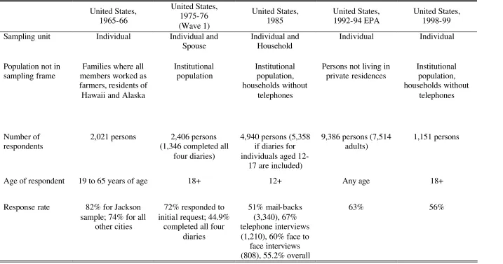
Details of each study are listed in Table 2. A comprehensive description and evaluation of

these American time use studies is given in Harvey and St. Croix (2005).

Time use theory based and standardized calibration for all heritage files

Computing new adjustment factors for the American Time Use Study (ATUS) will

improve subsequent research for two major reasons: first, for substantial analyses it is

important, that fundamental socio-demographic variables meet the given aggregates of

reliable demographic data such as the current population survey (CPS) or the Intercensal

Population Estimates of the U.S. Census Bureau. This increase in representativeness

concerning the socio-demographic structure of the sample also affects the representativeness

of the analysis of the episode data, if the socio-demographic variables are correlated with the

time use behavior. The selection of these variables is based on time use theory and the

individual-centered and social background-centered economic models discussed above.

Furthermore, time use-specific variables like the day of the week of an observation

should be considered in the adjustment factors as well, as these variables directly affect time

Merz and Stolze: Representative Time Use Data and Calibration of the American Time Use Studies 1965-1999 19/ 120

Table 2 American time use studies under investigation

United States,

1965-66

United States,

1975-76

(Wave 1)

United States,

1985

United States,

1992-94 EPA

United States,

1998-99

Sampling unit

Individual

Individual and

Spouse

Individual and

Household

Individual

Individual

Population not in

sampling frame

Families where all

members worked as

farmers, residents of

Hawaii and Alaska

Institutional

population

Institutional

population,

households without

telephones

Persons not living in

private residences

Institutional

population,

households without

telephones

Number of

respondents

2,021 persons

2,406 persons

(1,346 completed all

four diaries)

4,940 persons (5,358

if diaries for

individuals aged

12-17 are included)

9,386 persons (7,514

adults)

1,151 persons

Age of respondent

19 to 65 years of age

18+

12+

Any age

18+

Response rate

82% for Jackson

sample; 74% for all

other cities

72% responded to

initial request; 44.9%

completed all four

diaries

51% mail-backs

(3,340), 67%

telephone interviews

(1,210), 60% face to

face interviews

(808), 55.2% overall

Working with equally calibrated data will allow sensitivity analyses and disentangling

demographic changes vs. time use behavior changes. For this reason we will provide a

standardized calibration procedure for each of the American time use surveys.

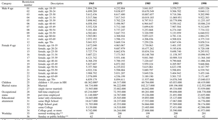
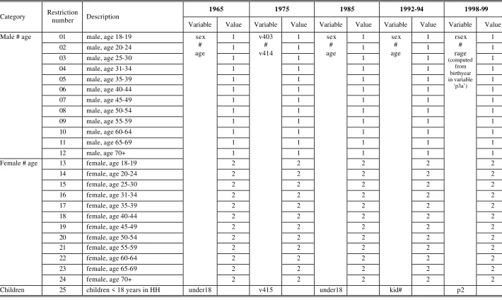
Aggregate characteristics for the heritage files

When selecting variables for the adjustment, several considerations must be made.

The structure of the sample should reflect the U.S. population with respect to major

socio-demographic data. Additionally, to improve the representativeness of the data, variables

should be chosen which are correlated with time use behavior. These may be

socio-demographic variables or technical variables of the time use survey itself (like a certain day

of the week). Choosing appropriate aggregates will support substantial analyses. We refer to

demographic backgrounds and individual characteristics based on human capital and other

performance characteristics within the time use analyses framework discussed. In addition,

we take the socio-cultural background of families and household characteristics into account.

The sample size and the nature of the calibration algorithm limit the amount of

restrictions in such a way that if there are a growing number of variables it will become more

likely that the sample may not provide observations for all the categories of the desired

aggregates. Furthermore, if a large number of restrictions exist, this may lead to very high

variances in the adjustment factors. Finally, the data has to be available in the sample files as

well as in the CPS-files (providing totals) for all of the specified years. When dealing with

five samples simultaneously, the selection of the optimal set of restrictions is difficult and

may vary from one which would have been chosen for a single calibration. Finding a

compromise between the desired detail of restrictions, practical requirements, and the

availability of data in all sample-files is a challenging task.

Considering the mentioned limitations, eligible structural variables in the heritage

files available for an adjustment to CPS key data and basic population estimates are:

•

Age (5-year-classes) crossed with gender

•

Educational attainment

•

Occupational status (full time/part time/unemployed, self-employed)

•

Marital status (single/married/divorced/widowed)

•

Number of children (below 18 years of age) living in household

Additionally to the structural data, following time use-variables can be used: