http://dx.doi.org/10.4236/jbise.2014.78050
Modeling Mechanical Patterns for Striated
Muscles
Valery B. Kokshenev
Departamento de Fisica, Instituto de Ciencias Exatas, Universidade Federal de Minas Gerais, Belo Horizonte, Brazil
Email: [email protected]
Received 9 April 2014; revised 25 May 2014; accepted 7 June 2014
Copyright © 2014 by author and Scientific Research Publishing Inc.
This work is licensed under the Creative Commons Attribution International License (CC BY).
http://creativecommons.org/licenses/by/4.0/
Abstract
Muscles show a surprisingly large variety of functions when they mechanically respond to differ-ent environmdiffer-ental requests. However, the in vivo workloop studies distinguish well only four pat-terns of skeletal muscles, producing positive, negative, almost zero and zero net works, that quali-fies them respectively as motors, brakes, struts, and springs. While much effort of comparative bi-ologists has been done in searching for muscle design patterns, no fundamental concepts under-lying such four primary patterns were established. In this interdisciplinary study, continuum me-chanics is applied to the problem of muscle structure in relation to function. The known ability of a powering muscle as whole to be tuned via natural (resonant) frequency to the efficient locomo-tion is now modeled through the non-linear elastic muscle moduli, controlling both the contrac-tion frequency and velocity. When incorporated in activated skeletal and cardiac (striated) mus-cles via the mechanical similarity between loaded and reaction forces, further exploration of elas-tic force patterns (borrowed from solid state physics) yields an explicit rationalization for cur-rently known locomotor muscle patterns. Besides explanation of the origin of allometric expo-nents derived for leg muscles in animals adapted to fast running and wing muscles in flying birds, the skeletal and cardiac muscles are patterned through the primary and secondary high power ac-tivities. Further applications are expected to be useful in designing of artificial muscles and mod-eling living and extinct animals.
Keywords
474
1. Introduction
The mechanical role of muscles varies widely with their architecture and activation conditions. Striated (skeletal and cardiac) muscles are diverse in their contractive interspecific and intraspecific functional properties ob-served among and within animal species, nevertheless, in all cases “the smaller muscles and muscles of smaller animals are quicker” [1]. After Hill [1] who first noted this generic feature of the design of skeletal muscles, their physiological adaptation, resulting in beneficial changes in muscle function, has been recognized by a number of investigators. For example, it was learned that long-fibre muscles commonly contract at over larger length ranges and relatively higher velocities producing the greatest muscle forces the lowest relative energetic costs [2]. Muscles having shorter fibres expose smaller length change, but their cost of force generation is rela-tively less, e.g. [3]. Searching for determinants of evolution of shape, size, and force output of cardiac and ske-letal muscle, a little is known about the regulation of directional processes of mass distribution [4] [5]. Although skeletal muscles grow in length as the bones grow, most studies only involve force increasing with respect to cross-sectional area. Following the idea that the muscle force production function is a critical evolutionary de-terminant [5], I develop a physical study of the muscle form adaptation to a certain primary activity with growth of size (length and cross-sectional area) under evident condition of the preservation of muscle shape.
When designing architecture of the striated muscle built from repeating units (fibres and sarcomeres) at least three distinct muscle activities should be distinguished [5]: the concentric contraction defined as the production of active tension while the muscle is shortening and performing positive work, the eccentric contraction defined as contraction during lengthening performing negative work in a controlled fashion, and the isometric contrac-tion when the muscle force output is produced without changing of length and performing almost zero or zero net work. The corresponding mechanical work patterns called by Russel et al.[5] as “concentric work” and “eccentric work” (that might be extended here by “isometric work”) were carefully studied via in vivo mea-surements of length-force cycling (workloops) of individual skeletal muscles in active animals. Presented (in Figure 3 in [6]) by the pectoralis in flying birds, leg extensors in running cockroaches, gastrocnemius in the level running turkey, and intrinsic wing muscles in insects, the corresponding muscle locomotor patterns are known as the motor, brake, strut and spring muscles [6].
The seminal research by Hill [1] on dynamics of electrically stimulated isolated muscles was restricted to a single isotonic shortening. The studies of the relevant motor function resulted in famous force-inverse-velocity master curve presenting the major dynamic constraint of all real (slow-fibre, fast-fibre, and superfast) muscles [7]
and computationally modeled muscles, e.g. [8]. Besides, other two fundamental rules of muscle dynamics were noted by Hill [1]. Examining hovering humming and sparrow birds, he recognized that the “frequencies of wings are roughly in inverse proportion to the cube roots of the weights, i.e. to linear size”. Moreover, because the linear proportionality between the stroke period
T
and body lengthL
was equally established in in vivo and electrically stimulated isolated muscles, the corresponding frequency-inverse-length scaling rule1 1 1
m m
T− ∝L− L− , shown for a given muscle m, is likely more universal than previously appreciated and asso-ciated with the nervous control. Second velocity-inverse-length Hill’s constraint states that “the intrinsic speed of muscle has to vary inversely to length”, i.e. 1
m m
V ∝L− . Both Hill’s scaling rules still remain a challenge to viscoelastic models of transient-state muscle mechanics and other theories of muscle contraction, e.g. [9].
In the present paper, I develop an integrative theoretical approach to the problem of active forces, mechani-cally adapted design, and contractive linear and non-linear dynamics of striated muscles. Instead of Hill-type modeling of in vitro motor function (e.g. [3]), brake function (e.g. [2] [12]), and strut function (e.g. [14]), or study of muscle design by means of simulation of phenomenological force-length and/or force-velocity con-straints [8], the powerful method of continuum mechanics generally providing macroscopic characterization and modeling of soft tissues (e.g. [15] [16]) is employed. As a further exploration of the elastic force patterns, I pro-pose a self-consistent depiction of the three dynamically-distinct point characteristics of typical in vivo force- length loops of the naturally activated skeletal muscles. Unlike the earliest elastic theories based on minimiza-tion of energy, I develop the physical concept of similarity between the force output and reacminimiza-tion active elastic forces that permits one to avoid the molecular-scale details of the muscle activation process. The theory is vali-dated by a comparison to phenomenological scaling rules including both mentioned Hill’s dynamic constraints and therefore may be hopefully helpful in designing artificial muscles [15] and modeling living and extinct or-ganisms [17].
2. Theory
2.1. Theoretical Background
2.1.1. McMahon’s Scaling to Body Weight
The engineering models by McMahon [18] [19] develop previous Hill’s approach to the problem of scaling quantities of animal performance to body weight W =Mg. Using Hill’s geometric similarity models [1] [19]
equally applied to animal body, long bone, or individual muscle, each one was approximated by a cylinder of longitudinal length
L
and cross-sectional areaA
(or diameter D A). Moreover, the assumption on the weight-invariance of for the tissue density was adopted, namely0
. tiss
M W AL
ρ = ∝ (1)
In mammalian long-bone allometry, this invariant was verified and observed with a high precision [20]. Me-chanical models of bending bones and shortening muscles were introduced by McMahon via the weight-inva- riant elastic modulus Etiss, tissue stress σtiss and strain εtiss, namely
0
, with and .
tiss
tiss tiss tiss
tiss
F L
E W
A L
σ σ ε
ε
∆ ∆
= ∝ = = (2)
Here ∆ = −L
(
L L0)
is the length change accompanied by the force change ∆F(
= −F F0)
counted off from the resting length L0.While searching for functional mechanical patterns of biological systems determined by maximal forces using Equation (1) and Equation (2), the maximal-amplitude stress/strain scaling relations
(max) 1 3 (max) 1 4 (max) 1 5
, , and ,
geom W elast W stat W
σ
∝σ
∝σ
∝ (3)could be readily derived from McMahon’s geometric (isometric elastic stress), elastic (buckling elastic stress) and static (bending elastic stress) similarity models distinguished through McMahon’s scaling relations
2 3 1 2
, , and .
geom elast stat
L D L ∝D L ∝D (4)
Instead, the maximum stress and strain
(max) (max) 0,
tiss tiss W
σ ∝ε ∝ (5)
were postulated (in Table 4 in [19]) thereby groundlessness extending McMahon’s exact result for the mean stress (mean) 0
elast W
σ ∝ , obtained within the static stress similarity model (see Figure 1 in [19]). The improved self-consistent maximal stresses shown in Equation (3) follow straightforwardly from McMahon’s cross-sec- tional areas
( ) 2 3 ( ) 3 4 ( ) 4 5
, , and ,
isom buck bend
geom elast static
A ∝W A ∝W A ∝W (6)
476
The patterns of long bones are generally driven by the peak muscle forces, but not by gravity, as repeatedly noted by many authors, proven [20] and exemplified by all mammals as whole [21]. Nevertheless, one amazing case of the experimental evidence of McMahon’s elastic similarity is due to limb bones in African elephants which, in contrast to Asian elephants, are most likely adapted for axial bone compression, influenced by gravita-tional reaction forces [21].
Although the evolution of locomotor trends of terrestrial giants are likely driven by body weight [22], the idea on the origin of locomotion patterns of animals (running, flying, and swimming) based on minimization of use-ful energy in the gravitational field [23], was also confronted with the new idea of maximum body efficiency in the muscular field [24].
2.1.2. Muscle Shape and Structure
After Alexander [25], the physiologic cross-sectional area A0m (PCSA) of the isolated skeletal muscle m of mass Mm composed of
N
bundles of masses mi was commonly estimated, e.g. [26], with the help of the cylinder-geometry relation Ai =mi ρmLi , where ρm is the muscle density and Li is directly measured mus-cle fibre length. The spindle-like shape of the musmus-cle as whole organ was therefore determined by the musmus-cle PCSA, namely0
1 0 1 0 1
1 1
since and , hence ,
N N N
m i
m i m i
i m m i m m i i
M m
A A M m
L L M L
ρ
= = =
=
∑
= =∑
=∑
(7)As shown [25] [26], the sum of areas of the muscle and the muscle length L0m of the parallel-linked contrac-tible subunits is described statistically by the length-unversed sum weighed by masses. Such a simplified (coarse-grained) characterization of the muscle structure generally ignores the arrangement of muscle fibres rel-ative to generated force axis, distinguished by pinnate angles.
In scaling models, the evolution of the muscle structures across different-sized animals of body mass
M
is observed statistically via allometric exponents am, lm, and αm determined by common rules [25] [27] [29]:1
0 , 0 , and ,
m m m
a l
m m m m m
A ∝M L ∝M M ∝M +α (8)
where the muscle mass index αm plays the same role as Prangel’s index β in bones, as noted in [30]. When the muscle-density invariance employed implicitly in Equation (7) and specified in Equation (1) is applied to different skeletal muscles, the muscle shape approximated by cylinder geometry is also preserved. Consequently, the muscle functional volume
0 0
0 0 0
0
, with ,
m
m m m m m m m
m M
A L A L ρ ρ M M
ρ
= = = ∝ (9)
holding in all muscle activities, plays the role of the muscle mechanical invariant. This statement is ensured by the functional variation of density ∆ρ ρm m not exceeding 5% [28]. Hence, the function-independent mus-cle-shape constraint[13]
1
m m m
a +l = +α (10)
straightforwardly follows from Equation (8) and Equation (9). Likewise the case of hindlimb mammalian bones of the mean structure (exp) (exp)
2 0.752
b b
a = d = , (exp)
0.298
b
l = , and (exp)
0.04
β = [20] [30], Equation (10) is also
empirically observable in muscle allometry (see further analysis inTable 5).
2.2. General Muscle Characterization
2.2.1. Maximal Force and Stress
Using the in vivo workloops, the muscle locomotor patterns can be generally specified regardless of details of activation-deactivation conditions. In Figure 1, the linear-slope characteristics L1m can be introduced in the force-length cycling by the length-point conditions: L2m<L1m<L3m ≈L0m , for the motor function,
2m 1m 3m
L >L >L , for the brake function, and by L2m L1m L3m ≈L0m, for the strut function showing nearly isometric muscle contractions.
Moreover, such a qualitative general characterization of the activated individual muscle m of resting length
0m
L can be rationalized on the basis of common two-point force-length description, namely
( )exp
( )
(max) ( )exp( )
2 2 and 1 1 ,
musc m musc m musc m m
Figure 1. The qualitative analysis of the in vivo muscle force-length data. The muscle motor function is presented by gastrocnemius powering during shortening in uphill running turkey (inset a, adapted from [31]). The lateral gastrocnemius and plantaris act as brake (inset b) and strut (inset c) in hop-ping tammar wallabies [28]. The solid (and dashed) arrows indicate rasing (and decreasing) of the exerted force near its maximum magnitude Fmax, dis-tinguished by the turningpoint 2. The regions of the linear force-length do-main are displayed by the force change ∆F1m and length change ∆L1m, es-timated from point 1 as the starting datapoint of the force enhancement F1m
with length L1m, achieved at the optimum contraction velocity Vopt and
frequency. Similar to cyclic pendulum, the activated muscle is expected to pass though point 3 with maximum contraction velocity Vmax at resting
length L0m, with moderate force F3m. Inset d: The resulted intrinsic force generated by the powering shortening (motor) or lengthening (brake) muscle, exemplified by Fmax, is due to a superposition of the production force output
prod
F and elastic forces, reaction passive Fpass and active Fact (see also
text below Equation (16)).
introduced by the maximum force (max) 2m
F and the optimum muscle length [32] [33] L1m. The instant dynamic length Lm =L1m± ∆L1m is counted off from the characteristic point L1m via the optimum length change ∆L1m shown in Equation (11) and Figure 1 for all locomotory functions.
First, the linearization of the in vivo muscle force-length curve allows one to determine the trial peak stress and strain by
(max) (max) (max) (1max) (max)
1 2 1
2 2
and , with .
musc m
musc musc m m m
m m
F L
L L L
A L
σ = ε =∆ ∆ = − (12)
The corresponding force change ∆Fmusc(max) observed near the optimum force F1(mmax) provides
(max) (max)
( )
(max) (max) (max)1 1 1
musc musc m musc m musc m
F =F L + ∆F =F +K ∆L (13)
that in turn determinates effectivemuscle stiffness K2m and effective modulus E2m, namely
( )
( )
( ) ( )
( )
( ) ( ) ( )
( ) ( )
max max max
max max 2 max
2 max max 2 max
max 2
1 1
d
, and ,
d
musc musc musc m musc
musc m musc musc m
m Fm m musc m musc
F F F A
K K E E E
L L F L
σ
ε
∆ ∆
≡ = ≈ = ≡ =
478
following from Equation (12) and Equation (13).
2.2.2. Active Stiffness and Resonant Muscle Mechanics
Secondly, treating the maximum-force crossover state as the generic transient-neutralstate [30], the resonant frequency (max) 1
2 1Tmusc Tm
−
= related to point 2 in Figure 1 and associated with maximum efficiency of muscle cycling, e.g. [34], can also be introduced as natural frequency[19] [34], namely
( ) ( ) ( )
( )
1 2 max
max max
1 2
2 max
0 2 2
1
2π m musc musc musc .
m
m m musc m m
E
K E F
T
M ρ F L L
− ∆ ∝
(15)
One can see that Equation (15) yields first Hill’s frequency-inverse-length constraint discussed in Introduction. However, the following three observation conditions of this constraint are required: 1) the preservation of dy-namic functional volume(see Equation (9)), 2) the weight-invariance of the elastic modulus Emusc(max), and 3) the validation of force similarity between the exerted force Fmusc(max) and its change ∆Fmusc(max) (see Equation (13)). Therefore, the muscle force-similarity principle, implying a coexistence of all forces in biomechanically equiv-alent states [30], can be formulated as
.
musc musc prod elast elast
F ≅ ∆F ≅F ≅F ≅ ∆F (16)
Here the active elastic force ∆Felast (shown schematically in the inset d (see Figure 1 as Fact) is also in-cluded1. The total transient-state elastic force Felast is the superposition of common passive elastic force Fpass provoked by external loads and active elastic force ∆Felast caused by the production force Fprod.
Given that the peak active muscle stress σm always exceeds the corresponding passive stress, e.g. [14], in further I focus on transient states in the fully activated muscle (restricted by points 1 and 2 in Figure 1) and de-scribed by . elast m m m m m F L E A L
σ =∆ = ∆ (17)
Unlike the trial peak stress in Equation (12), σm is the true intrinsic elastic stress in a certain, non-specified transient dynamic state. This reveals elastic force change near the maximum amplitude
m
elast m m m m m
m L
F F K L E A
L
∆
∆ ≡ ∆ = ∆ = (18)
and in turn provides the corresponding activemuscle stiffness
. m m m m A K E L
= (19)
The underlying mechanical sarcomere elastic stiffness Ks is related via the muscle-volume average, namely
( )
31
d ,
m s m m
m m
K K r r
A L
=
∫
(20)originated from end-to-end intercellular overlapping [12] [35]. The muscle energy change
2
2 m
m m m m m
m L
U K L E A
L
∆
∆ ∆ ≅ (21)
stored or released during active-period contraction provides the mechanical cost of energy
.
m m
m m m
m m
U L
CU E A
L L
∆ ∆
= ≅
∆ (22)
These relations demonstrate how the observable mechanical characteristics can be linked to the underlying muscle elastic forces using the force-similarity principle formulated in Equation (16). In turn, the contraction
1The correspondence sign ≅ indicates that though the involved physical characteristics belong to the same mechanical state, they may
velocity
( )
1 0 d( )
d( )
d d
m
m
t m m m
m m
m t t m
L t L t L
V V t dt
t t t T
∆
=∆
= ≡ ≅
∆
∫
(23)is defined by the instant velocity Vm
( )
t averaged over activation time ∆tm. 2.2.3. Fast and Slow Activated MusclesAccording to the most general classification of diverse muscles, three types are conventionally distinguished: red (slow fibre) muscles, white (fast fibre) muscles, and intermediate type, mixed fibre muscles. Although col-lective mechanisms of muscle contractions are poor understood, e.g. [36], physically, two limiting situations of the dynamic accommodation of local forces generated by cross bridge attachments can be generally rationalized. As schematically drawn in the inset d in Figure 1 for an activated muscle, the dynamic process of equilibration between the production intrinsic forces and external loads (not shown) is followed by the spatiotemporal relaxa-tion of elastic forces. For the simplest case of slow muscles, the dynamic equilibration occurs via the slow chan-nel of relaxation, supposedly common for both active, Fprod(slow), and passive elastic forces. Since passive forces in solids are short of range [37], both the forces are proportional to muscle surface. In contrast, it is plausible to adopt that in fast muscles the fast-twitch fibres transmit the locally generated forces in all directions, i.e. along and across fibres, resulting in the overall maximum force output Fprod(fast) to be linear with dynamic muscle vo-lume. Basing on such a generalized physical picture, a function-independent and regime-independent characte-rization of the force production function, namely
(fast) and (slow) , with 1, 2, and 3,
prod rm rm prod rm
F ∝A L F ∝A r= (24)
is proposed through the force-size scaling rules, for all three distinct states shown in Figure 1, hereafter distin-guished by symbol r.
The linear-displacement regime with
∆
L
L
widely adopted among biologists for overall dynamic charac-terization, is discussed in Equation (2) that results in the weight-independent strain, that may shed light on stress postulated in Equation (5). The corresponding optimum-velocity regimer
=
1
, attributed to the instantlength-independent elastic strains, ( ) 3 0
opt
m Lm Lm Lm Lm
ε
= − ∝ with Lm lying between L1m and L3m≈L0m, is now introduced by scaling equations( ) ( ) 1 ( ) ( ) 0
1 , 1 , with 1 ,
fast opt slow opt
m fast m m slow m m m
E =E ∝L E =E ∝L ∆L L (25)
characteristic of the fast and slow muscles. Such a muscle description follows from the principle of similarity (see Equation (16)) between the active elastic force 1 ( )opt 1 1 1
m elast m m m
F F E A ε
∆ = ∆ = (see Equation (18)) and
cor-responding production force (see Equation (24)). The optimum-force and optimum-velocity muscle mechanics is rationalized below inTable 1 and then tested by empirical data.
Likewise, the bilinear-displacement moderate-velocity regime
r
=
2
introduced by the dynamic lengthchange 2
2m m 1m m
L L L L
∆ = − ∝ , with Lm lying between L2m and L1m, and the maximum active elastic force
(max) (max)
2m elast 2m 2m 2m
F F E A ε
∆ = ∆ = (see Equation (18)) results in the maximal elastic moduli
(max) ( ) 0 (max) ( ) 1 2
2 , 2 , with 2 ,
fast slow
fast m m slow m m m m
E =E ∝L E =E ∝L− ∆L ∝L (26)
adjusted with the muscle production function on the basis of force similarity principle. Finally, the trilinear high-velocity regime
r
=
3
is suggested by the moderate elastic muscle force determined by( ) ( ) 1 ( ) ( ) 2 3
3 , 3 , with 3 .
mod fast mod slow
fast m m slow m m m m
E =E ∝L− E =E ∝L− ∆L ∝L (27)
This condition specifies point 3 in Figure 1, along with the underlying cubic-power muscle displacements
3m L
∆ scaled by dynamic Lm lying above or below the characteristic length L3m in any muscle acting as mo-tor, brake or strut.
2.3. Muscle Functions
480
work exerted by elastic bending forces. Given that the elastic force patterns coincide for bending and torsion
[image:8.595.81.538.209.342.2][30], both kinds of unpinnate and uni-pinnate skeletal muscles, having respectively close to zero and non-zero fixed pinnate angles, may be expected to be structured by the same motor function. The specific-function me-chanical characterization is described in Appendix B and results are summarized in Table 2.
Table 1. General mechanical characteristics of the striated muscles tuned to linear-displacement dynamic regime scaled to
dynamic fibre length Lm=L1m. The mixed-fibre scaling dynamic exponents (shown in the last column) are modeled by the common means for the fast-muscle and slow-muscle exponents (established in the second and third columns), following from the rule Fmix FfastFslow ; Am and Lm are attributed to the stabilized dynamic muscle geometry constrained by
muscle volume Equation (9).
Optimum muscle characteristics, Equation Fast fibres Slow fibres Mixed fibres
Optimum length change, ∆L1m, Equation (25) Lm Lm Lm
Production force, ∆F1m, Equation (16), Equation (18), Equation (25) A Lm m Am
1 2 m m
A L
Optimum stiffness, K1m=E A1m 1m L1m , Equation (19) Am
1 m m
A L− 1 2
m m
A L−
Optimum elastic stress, σ = ∆1m F1m A1m, Equation (17) Lm
0 m
L 1 2
m
L
Contraction frequency, 1
1m 1m 0m 1m
T− E ρ L , Equation (15) 1 2
m
L− 1
m
L− 3 4
m
L−
Optimum velocity, 1 ( ) opt m musc
V =V , Equation (23) 1 2
m
L 0
m
L 1 4
m
L
Optimum power, P1m=F V1m 1m
3 2 m m
A L Am
3 4 m m
A L
Table 2. Scaling to mass of mechanical characteristics of muscles adapted to different locomotor functions. The allometric
exponents related to animal's body mass (via Equation (8)) are presented in terms of muscle mass index αm. The powering
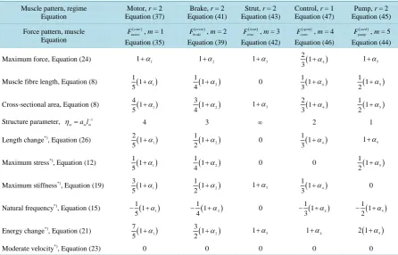
individual muscles m=1, 2,3, and 5 are tuned to the maximum-force bilinear dynamic regime r=2 (described in Equa-tion (26)) and the control muscle m=4 acts in the linear regime r=1 (Equation (25)). *)The data shown only for the fast-fibre muscles. Other data are equally applied to fast, slow and mixed-fibre muscles.
Muscle pattern, regime Equation
Motor, r = 2 Equation (37)
Brake, r = 2 Equation (41)
Strut, r = 2 Equation (43)
Control, r = 1 Equation (47)
Pump, r = 2 Equation (45)
Force pattern, muscle Equation
(conc)
motor
F , m = 1 Equation (35)
(eccen)
brake
F , m = 2 Equation (39)
(isom)
strut
F , m = 3 Equation (42)
(sprin)
contr
F , m = 4 Equation (46)
(card)
pump
F , m = 5 Equation (44)
Maximum force, Equation (24) 1+α1 1+α2 1+α3 ( 4)
2 1
3 +α 1+α5 Muscle fibre length, Equation (8) ( 1)
1 1
5 +α ( 2)
1 1
4 +α 0 ( 4)
1 1
3 +α ( 5)
1 1 2 +α
Cross-sectional area, Equation (8) ( 1)
4 1
5 +α ( 2)
3 1
4 +α 1+α3 ( 4)
2 1
3 +α ( 5)
1 1 2 +α
Structure parameter, 1 m a lm m
η = −
4 3 ∞ 2 1
Length change*), Equation (26) ( )
1
2 1
5 +α ( 2)
1 1
2 +α 0 ( 4)
1 1
3 +α 1+α5
Maximum stress*), Equation (12) ( )
1
1 1
5 +α ( 2)
1 1
4 +α 0 0 ( 5)
1 1 2 +α
Maximum stiffness*), Equation (19) ( )
1
3 1
5 +α ( 2)
1 1
2 +α 1+α3 ( 4)
1 1
3 +α 0
Natural frequency*), Equation (15) ( 1)
1 1 5 α
− + ( 2)
1 1
4 α
− + 0 ( 4)
1 1 3 α
− + ( 5)
1 1
2 α
− +
Energy change*), Equation (21) ( )
1
7 1
5 +α ( 2)
3 1
2 +α 1+α3 1+α4 2 1
(
+α5)
[image:8.595.90.537.424.710.2]3. Results
Assumptions and Predictions
The following assumptions are made regarding elastic striated muscles in fully activated states:
1) The powering individual muscles considered at macroscopic scale are treated as regime-dependent homo-geneous solid-like organs. Within the scope of continuum medium mechanics, the macroscopic coarse-grained description ignores details of heterogeneous microstructure, including those resulting in pinnate angles.
2) When activated under different boundary loading conditions, the muscles do not undergo changes in shape and whole volume. The emerging muscular active-force fields [24] [38] follow the same patterns as passive elastic-force fields known in continuum medium mechanics of solids.
3) The mechanical similarity between the extrinsic forces exerted by the muscle and intrinsic elastic reaction forces, established above as the observation condition, can provide dynamic similarity features (for contraction velocities and frequencies), which can be theoretically and experimentally observable, at least in biomechani-cally equivalent states.
4) The natural ability of the non-linear elastic tuning of fast and slow muscles [34] can be characterized by the regime-dependent elastic moduli sensitive to evolving dynamic observable characteristics, e.g. the muscle length change.
One can deduce from Table 1, that the mechanical characterization of slow, fast and mixed muscles attributed to the linear-displacement regime
(
r=1)
is shape-dependent.In Table 2, the scaling rules driving mass distribution in a given muscle m are provided in terms of the muscle mass index αm. For example, the solution for the muscle-fibre length scaling exponent lm= +
(
1 αm)
5 specified for the motor function(
m=1)
follows from the muscle scaling Equation (8) and muscle motor pat-tern in Equation (37), both indicated in Table 2. [image:9.595.90.537.520.719.2]In Table 3, the scaling rules shown in Table 2 are compared with those for the optimal-force state related to the exponents
[
a1m,l1m]
and moderate-force state related to[
a3m,l3m]
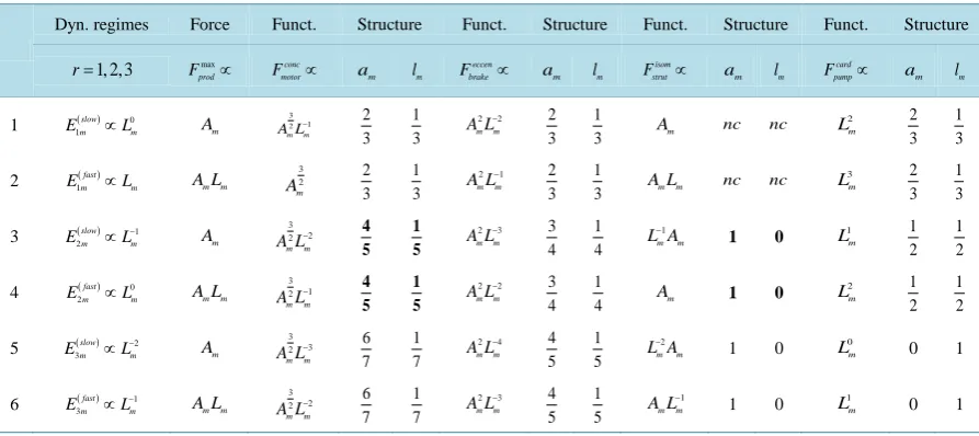
. The dynamic characteristics of dis-tinct-velocity contractions are predicted in Table 4.Table 3. Locomotor functions predicted by dynamic structured for slow and fast striated muscles tuned to distinct dynamic
regimes. The primary functions
(
r=2)
are shown by bold exponents. The analysis of functional muscle structures made in terms of elastic-force patterns: the active-muscle optimum-velocity(
r=1)
, moderate-velocity(
r=2)
, and high-velocity(
r=3)
dynamic regimes are described in the first column via the muscle elastic moduli Erm (see Equations (25)-(27)) and specified by slow and fast force output (Equation (24)), shown in the second column. The third and next odd columns show the elastic force functional scaling in concentric, eccentric, isometric, and pump contractions. Unlike Table 2, the corres-ponding solutions to scaling equations underlaid by the force similarity principle Equation (16) are shown for simplicity with0 rm
α = . Notation: nc indicates non-conclusive solution.
Dyn. regimes Force Funct. Structure Funct. Structure Funct. Structure Funct. Structure
1, 2,3
r= max
prod
F ∝ conc motor
F ∝ am lm eccen brake
F ∝ am lm isom strut
F ∝ am lm card pump
F ∝ am lm
1 ( ) 0
1 slow
m m
E ∝L Am
3 1 2 m m
A L− 2
3 1 3
2 2 m m
A L− 2 3
1
3 Am nc nc
2 m L 2 3 1 3
2 1( ) fast
m m
E ∝L A Lm m
3 2 m
A 23 13 A Lm2 m1
− 2
3 1
3 A Lm m nc nc 3 m L 2 3 1 3
3 ( ) 1
2 slow
m m
E ∝L− Am 3
2 2 m m
A L− 4 5
1 5
2 3 m m
A L− 3 4
1 4
1 m m
L A− 1 0 L1m
1 2
1 2
4 ( ) 0
2 fast
m m
E ∝L A Lm m 3
1 2 m m
A L− 45 15 A Lm2 m2
− 3
4 1
4 Am 1 0
2 m L 1 2 1 2
5 ( ) 2
3 slow
m m
E ∝L− Am 3
3 2 m m
A L− 67 17 A Lm2 m4
− 4 5 1 5 2 m m
L A− 1 0 0 m
L 0 1
6 ( ) 1
3 fast
m m
E ∝L− A Lm m 3
2 2 m m
A L− 67 17 A Lm2 m3
− 4 5 1 5 1 m m
A L− 1 0 1 m
482
Table 4. Dynamic characterization of the red (slow) and white (fast) striated muscles in the optimum-, moderate-, and
max-imum-velocity dynamic regimes r=1, 2, and 3 described in Table 3. Predictions are made on the basis of equations indi-cated in the table generalized over different dynamic regimes.
Dynamic regime Optimum
(
r=1)
Moderate(
r=2)
Maximum(
r=3)
Muscle type slow fast slow fast slow fast
Natural frequency, Equation (15), 1 rm
T− ∝ 1
m
L− 1 2
m
L− 3 2
m
L− 1
m
L− 2
m
L− 3 2
m
L−
Contraction velocity, Equation (23), Vrm∝
0 m
L 1 2
m
L 1 2
m
L− 0
m
L 1
m
L− 1 2
m
L−
Some consequences of the proposed muscle scaling dynamic theory are:
1) The peak forces generated in all regimes scales as muscle volume or PCSA, respectively, in fast or slow muscles.
2) A general, function-independent mechanical description of the striated muscle activated in the lin-er-displacement regime is predicted for each type of muscles (Table 1).
3) The muscle-type independent locomotor functions and related mechanical and dynamic characteristics of the striated muscle activated in the bilinear regime are predicted (Table 2).
4) The muscle-type independent varied dynamic structures are predicted for all muscle regimes and functions (Table 3).
5) The function-independent dynamic scaling characteristics are obtained in Table 4 for all type of muscles. In what follows, all theoretical findings are tested by available from the literature data.
4. Analysis and Discussion
Aiming to shed light on some important problems in the field of muscle dynamics, let me cite Louis Sullivan quoted in [5]: “What determines the shape, size, and force output of cardiac and skeletal muscle?”. Broadly, within the provided coarse-grained description of conservative striated muscles, the proposed theory suggests that the size-dependent peak elastic forces, emerging during the force production preserving muscle shape, are responsible for the muscle patterns observed via the functionally adapted structures. Moreover, the peak force output, which is described through the corresponding elastic force, is therefore determined by the muscle vo-lume and cross-sectional area, respectively for white and red muscles, regardless of muscle functional speciali-zation.
4.1. Function against Structure
4.1.1. General Muscle CharacterizationBeing composed of bundles of muscle fibres and other contractible components (neural, vascular, and collagen-ous reticulum), the striated muscle is thought of as a heterogenecollagen-ous continuum medium transmitting the pro-duced tension internally and externally, e.g. [39]. Primarily, I address the problem of mechanical design of striated muscle to a general, function-independent characterization of the individual muscle organ loaded by tension, reaction, and gravity through tendons, ligaments, and bones. My non-energetic approach is physically grounded by the existence of linear force-length regions (shown by the solid arrows in the workloops in Figure 1) revealed in all in vivo workloops regardless of dynamic details of approaching to the peak exerted force
(max)
musc
F . Hence, the mechanical characterization of the maximum-force activated muscle arises from the muscle stiffness (max)
m
K underlaid by sarcomere stiffness (max)
s
K discussed in Equation (20). Consequently, all forces involved in muscle contraction following by active and passive elastic strains allow common mechanical de-scription (shown in the inset d in Figure 1) not depending on their biochemical, inertial, or reaction origin.
The analytical justification of Hill’s frequency-inverse-length constraint results from the analysis of Equation (15) that eventually requires the usage of the similarity between all intrinsic muscle forces, Equation (16). The
constraint 1 1
m m
T− ∝L− and other mechanical characteristics for slow muscles shown in Table 1 can be generally applied to steady-speed regimes of locomotion modes where all forces are generally equilibrated and controlled by slow-fibre muscles [40]. In the case of non-steady transient locomotion when fast-twitch fibres and nervous control are additionally requested [40], Hill’s first constraint transforms (by Equation (15) and Equation (25)) into a new one, Tm1 Lm1 2 1Vfast( )opt
− ∝ − ∝
maxim-al optimum speeds [41] [42] Vrun(max)Vfast( )opt ∝ L Lm.
Thereby, it has been demonstrated that the dynamic similarity establishes a link between the body-propulsion speed and locomotor-muscle contraction velocity, earlier described by Rome et al.[43]. Being united with the muscle-force similarity, both constraints lead to the mechanical similarity, as the basic principle explored in this research. More general approach to the problem of dynamic similarity in animal locomotion shows that the con-cept of mechanical similarity [24] and obtained above findings naturally follow from the key principle of ana-lytical mechanics applied to the resonant (in frequency and phase) efficient cyclic locomotion [38].
4.1.2. Maximum Force Output against Structure and Velocity
In muscle physiology, the functional effect of muscle conceptual architecture simply states that muscle force output is proportional to PCSA. It may seem that the proposed study of the adaptation of muscle structure via force production function is in qualitative agreement with this statement, because in both cases of fast and slow muscles exposed in Equation (24) the muscle force output is proportional to Am. Since a simplified treatment of the fast-muscle mechanics (in fact excluding other important dynamic variable Lm) leads to a widely adopted opinion that the size-independent peak stress Fprod( )exp Am, validating for the particular case of slow muscles (Table 1), is generic for all types of muscle, as already discussed in Equation (5).
Although the proposal on scaling of the maximum production force (and active stress) with muscle size shown in Equation (24) is a challenge for further research, the provided fairly general physical grounds are sup-ported by empirical observations by Marden and Allen [44]. They statistically established that the peak force output in all biological (and human-made) motors falls into two fundamental scaling laws: 1) in fast-cycling motors, presented by flying insects, bats and birds, swimming fishes, and running animals the peak force scales as (motor mass)1 and 2) in slow-cycling motors, such as myosin molecules, muscle cells, and some (unspecified) “whole muscles” the force output scales as (motor mass)2/3; where the role of “motor mass” plays muscle (like fuel) mass. Within this context, the studied individual muscles are treated as complex biological motors, work-ing due to actomyosin linkages (cross bridges), interactwork-ing in both longitudinal and transverse directions [5] [13]. The fact that muscle motors were observed from sarcomere to whole muscle organ passing through the sin-gle-fibre level of muscle organization, makes a basis for the introduced below micro-macro scale correspon-dence.
The study of the in vivo force-length curves is provided here in terms of the three distinct characteristic points (shown in Figure 1) characterized by the force and velocity inequalities
2m 1m 3mand 2m 1m 3m.
F >F >F V <V <V (28) These three function-independent generic states are associated with the linear
(
r=1)
, bilinear(
r=2)
, and trilinear(
r=3)
muscle dynamics determined via the muscle elastic moduli Erm in Equations (25)-(27), re-spectively. The mechanical characterization of slow and fast striated muscles is therefore provided in terms of the maximum(
∆F2m)
, optimum(
∆F1m)
and moderate(
∆F3m)
active elastic-force changes developed at the measurable maximum( )
V3m , optimum( )
V1m , and moderate( )
V2m contraction velocities (Table 4). The sta-bilization of the generic dynamic states is expected to be ensured by muscle tuning to natural frequencies, scaled to the dynamic length Lrm and shown in Table 4.4.1.3. Muscle Functions against Size and Shape
Searching for answer on “what features make a muscular system well-adapted to a specific function?” [32], it has been communicated [13] that the natural conditions of stabilization of the moderate-velocity regime
r
=
2
, adjusted via the invariable fast-twitch fibre elastic moduli described here in Equation (26), result in muscle spe-cific primary functions directly observed through the adapted resting muscle length (see Figure 1 in [13]).Likewise [13], the elastic-force patterns, underlying concentric, eccentric, isometric, and cardiac contractions and determining eventually specific functions, are suggested, respectively in Equation (35), Equation (39), Equ-ation (42), and EquEqu-ation (44). The solutions to the muscle-force and muscle-shape constraints are accumulated in Table 2as patterned functions well distinguished through the muscle structure parameter
484
[34] during shortening (
m
=
1
,η =1 4), lengthening (m
=
2
,η =2 3), or oscillating near the “isometric” dynamic state (m
=
3
,η = ∞3 ), energy-saving state (m
=
4
,η =4 2), and high-pressure-resistant state (m
=
5
,η =5 1). The established lower structure parameter for the cardiac muscle (η η5< m, withm
≠
5
) is in accord with the de-scription by Russel et al.[5] that “the heart chamber, unlike skeletal muscles, can extend in both longitudinal and transverse directions, and cardiac cells can grow in length and width”. The scaling finding d lnL5=d lnA5 clearly indicates that the pump muscles may grow equally with mass in both along- and cross-sectional direc-tions. Within this context, the scaling analysis tells us that the locomotor skeletal muscles are expected to grow more in length than width.In Table 3, conceivable stable dynamic structures corresponding to muscle activity in different dynamic re-gimes are analyzed. As in the case of Table 2, the solutions to dynamic constraints follow from the similarity between the force outputEquation (16) and elastic-force patterns. The resulting dynamic states are considered in terms of the scaling exponents for the muscle dynamic structure
[
Arm,Lrm]
preserving muscle shape and vo-lume Equation (9). Other related observable mechanical characteristics are exemplified in Table 1 and Table 2. The major outcome of the analysis in Table 3 is that both slow-twitch and fast-twitch fibres belonging to the same muscle m should manifest concerted behavior coordinated by the dynamic active elastic forces and con-trolled by dynamic structure. As example, let us consider dynamic structure of the motor muscle (m
=
1
in Ta-ble 2) with the resting structure[
a0m =4 5,l0m =1 5]
presented by item 4 in Table 3. In the linear-displace- ment regimer
=
1
, the fast motor preserves the dynamic structure[
2 3,1 3 , that suggests the controllable]
spring as a secondary function for the motor. Likewise, the brakes and struts tuned to the linearly regime via the cycling frequency 11slow
T− or 1
1fast
T− (items 1 and 2, also described in Table 4) show the same multifunctional spring-type activity [13], as the secondary function. It is remarkable that the fast motors, brakes and struts being switched to the slow bilinear regime via 1
2slow
T− work as slow motors, brakes and struts preserving the same cor-responding dynamic structures (shown in item 3). When extended over other regimes, this finding also implies that even occupying similar dynamic volumes the slow-twitched fibres and fast-twitched fibres interact by dif-ferent ways producing distinct force output, as discussed in Equation (24). In the maximum-velocity regime
= 3
r
, the secondary function coincides with the primary function for the case of strut muscle (see items 5 and 6), whereas the brake muscle may efficiently work as motor. New secondary activities are exposed by the motor, which also may function as “the fastest motor”, determined by η6=( ) ( )
6 7 1 7 =6, and by the cardiac muscle, which fast-velocity action may suggest, say, a “sharp-heart” accommodation associated with η =0 0, formally opposed to that of the strut(
η3 = ∞)
.4.2. Direct Observations of Muscle Specialization
“If a muscle is specialized for a particular mechanical role how this is reflected in it architecture?” [45]. The proposed solution to stated problem is demonstrated below by the comparative analysis between the muscle ar-chitecture observed by allometric exponents and that predicted by the adaptation to a particular mechanical function.
4.2.1. Isolated Muscles in Hindlimb of Mammals and Birds
In Table 5 we analyze the morphometric data on the allometric exponents derived from the mean cross-sec- tional area A0(expm ) and length L(0expm) of four skeletal muscles in the mammalian hindlimb for 35 quadrupedal species of body-mass domain exceeding four orders in magnitude.
First, let us verify the cylinder-shape similarity of skeletal muscles described by Equation (9). The muscle mass index α0m estimated in Equation (10) via experimental data (exp)
0m
a and (exp) 0m
l is compared in Table 5 with the measured indexes (exp)
0m
α .
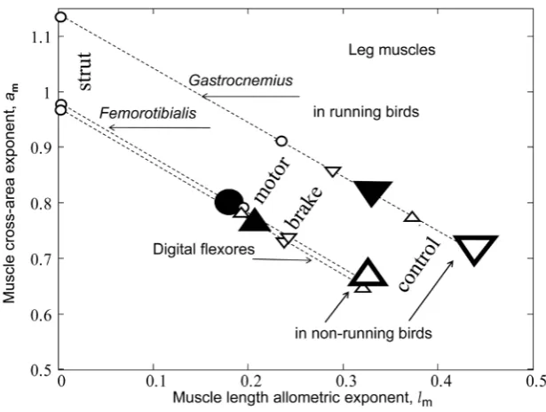
In Figure 2 and Figure 3, the method of determination of the primary mechanical function is illustrated: the adapted muscle structure is indicated by the appropriate theoretical point located most closely to the datapoint.
The found reliable estimates α0( )estm were used then in the muscle-function analysis in Figure 2 and Figure 3. The established small indices α0m generally validate the muscle biomechanics by proving a high-precision ob-servation of locomotory muscle patterns via muscle morphometry and functional physiology. This implies that the effect of biomechanical adaptation of muscle design to active elastic forces predominates over effects of bi-ological adaptation assigned to small (exp)
0m
α .
primary functions indicated in Table 5 are found with a high degree of certainty. Indeed, as illustrated in Figure 2, the deviations of distances measured along the dashed line, corresponding to a given muscle, between the da-tapoint and distant challengers for the primary function, from the smallest distance indicating the primary can-didate, always exceed the experimental uncertainty.
Thirdly, the found muscle mechanical specifications do not conflict with the physiological categorization es-tablished for joint extensors and flexors, which muscle structures are shown to be adapted to the brake and mo-tor functions via activation of eccentric and concentric elastic forces. The found structure parameter ηplant ≈18 indicates the foot support activity for plantaris as the primary function (Table 5) that is in accord with in vivo workloop presented in the inset c in Figure 1. As shown in Table 3, the struts are most conservative muscles
Table 5. The analysis of the allometric data by Pollock and Shadwick [26] provided on the basis of Equation (10) and Table
2. The shown statistical error is approximated by the symmetrized 95% confidence interval. The methodology of the analysis is illustrated in Figure 2. The primary functions found in Figure 2 and Figure 3 are described following Table 2, with
( )
0
est
m m
α =α . The overall muscle group
(
g=1)
is determined as the standard mean over all muscles. *)DDF includes indi-vidual flexor hallucis and flexor digitorum longus; SDF means superficial digital flexor.Individual mammalian
muscle
( )exp 0m
a ( )exp 0m
l ( )exp 0m
α η0m
( )
0 est m
α am lm Primary funct.
Gastrocnemius
(and soleus) 0.77 ± 0.02 0.21 ± 0.02 −0.03 3.7 −0.02 0.78 0.20 motor, m=1 Deep digital
flexor (DDF)*) 0.85 ± 0.03 0.18 ± 0.02 0.03 4.7 0.03 0.82 0.21 motor, m=1
Common digital
extensor (CDE) 0.69 ± 0.04 0.24 ± 0.02 −0.07 2.9 −0.07 0.70 0.23 brake, m=2
Plantaris (SDF) 0.91 ± 0.04 0.05 ± 0.04 −0.03 18 −0.04 0.96 0.00 strut, m=3
Ankle-joint
muscle group 0.81 ± 0.03 0.17 ± 0.03 −0.03 4.8 −0.03 0.78 0.19 motor, g=1
Figure 2. The indirect observation of the primary activity of mammalian plantaris.
The solid symbol is the datapoint [26] presented in Table 5 and the bars indicate ex-perimental error. The open symbols are theoretical estimates for stable dynamic struc- tures established for the motor, brake, strut, or control functions described in Table 2, with 0( )est
m m
486
Figure 3. The observation of the primary mechanical function in some isolated
indi-vidual muscles in mammals. The analysis and notations correspond to those in
Fig-ure 2. The experimental (and theoretical) data for gastrocnemius, DDF (deep digital
flexor), and CDE (common digital extensor) are shown, respectively, by the closed (and open) inverted triangles, regular triangles, and circles. All the data are taken from Table 5.
no changing their support function in non-linear regimes. In contrast, the gastrocnemius in mammals manifests their motor, strut, and brake functions in, respectively, uphill, level, and incline running of animals. Through the motor adapted structure with ηgast ≈η1=4, the analysis in Figure 3 establishes the motor activity for gastroc-nemius as the primary function naturally selected for the significant mechanical task of uphill running exploring the bilinear muscle dynamics. The effective trilinear gastrocnemius-displacement dynamics is most close to the brake-like activity
(
η6=6)
, attributed to the secondary function of the motor experimentally observed in ga-strocnemius of incline running turkey [31] and hopping tammar wallabies [28].In Figure 4, the overall muscle peak stress data measured in limb muscles of animals in strenuous activity, reviewed by Biewener [29], are re-examined and re-analyzed accounting for the primary functions of hindlimb muscles established in Table 5.
The uphill-motor specialization of gastrocnemius is independently supported by the compressive-stress anal-ysis made in Figure 4 for fast running, jumping, and hopping mammals. The stress scaling exponents
( )
sm predicted for the motor(
s1=1 5)
, strut(
s3=0)
, and control(
s4 =0)
functions are shown to be distin-guishable in work-specific mammalian muscles described in Table 2. Hence, although the overall-function data by Biewener [29] indeed expose almost weight-independent muscle stress, earlier postulated by McMahon in Equation (5) and only in part justified here by the slow-fibre muscles (Table 1) and strut muscles (Table 2), the analyses in Figure 4 demonstrates how the function-specific muscle stress may serve as a new tool for the direct observation of muscle specialization generally ignored in all previous overall-function analyses.I have also investigated an interesting question: whether the primary function established for a certain leg muscle in mammals specialized to fast running coincides with that for the same muscle in birds? The pioneering data on individual leg muscles in 8 running birds, ranging in size from 0.1 kgquail to 40 kg ostrich, are analyzed in Table 6 and Figure 5.
In non-running birds, the legs are designed to control the ground locomotion (Figure 5), whereas their wings may share motor and brake functions (Table 3), in accord with that reviewed by Dickinson et al.[6].
Figure 4.Thequalitative study of the in vivo data on the peak stress in
indi-vidual leg muscles of animals in strenuous activity. The symbols employed above in Figure 2 and Figure 3 are extended by the open circles (triceps) for the data on peak muscle stress taken from Table 1 in [29], with the exclusion of the slow-mode data on cantering goat and trotting cat. The data [46] on the activated isometric stress in isolated white rabbit tibialis are added. The dashed line shows the brake-functional stress indicated by the stress scaling exponent s=1 4. The solid lines are drawn by 115⋅M1 5, for the motor function, and by 215 kPa, for the strut and spring functions. All coefficients are adjusted by eye.
Table 6. The analysis of the allometric data by Maloiy et al.[47]. The shown large error is due to relatively wide confidence
limits. The mean exponents 0( )
est m
l are estimated via Equation (10). The overall muscle group is determined as the standard mean over all muscles. The indicated primary functions and active elastic forces are described by the evaluated dynam-ic-structure exponents a2m and l2m found as most close to the experimental resting-volume data on (exp)
0m
a and ( )exp 0m l and
therefore assigned to regime r=2 (Table 2).
Running birds ( )exp 0m
a ( )exp
0m
α ( )
0 est m
l ( )exp ( ) 0 0
est
m m
a l a2m l2m
Primary function (force)
Gastrocnemius 0.81 ± 0.14 0.14 0.33 2.5 0.85 0.29 brake (eccentric)
Digital flexors
(DF) 0.76 ± 0.22 −0.0.3 0.21 3.6 0.78 0.19 motor (concentric)
Femorotibialis 0.80 ± 0.12 −0.02 0.18 4.4 0.78 0.20 motor (concentric)
[image:15.595.87.539.614.722.2]488
Figure 5. The analysis of the primary mechanical functions for leg muscles in
run-ning and non-runrun-ning birds. The measured (and estimated) data taken from Table 6
(and Table 2) for gastrocnemius, femorotibialis, and digital flexors are shown by the closed (and open) inverted triangles, circles, and regular triangles, respectively. The semi-open triangles are the data by Bennett [27] for non-running birds.
4.2.2. Micro-Macro Scale Correspondence
There are many striking examples when skeletal muscles expose adaptation to a specific function, e.g. [3] [48]. The striated muscles anatomically suited to concentric or eccentric work [2] are structurally distinct having, re-spectively, long thin cells or short wide cells [5]. This observation suggests the microscopic level of muscle-cell adaptation introduced here by
(conc) (ecent)and (ecent) (conc)
cell cell cell cell
A >A L >L (29)
for the cellular cross-sectional area Acell and length Lcell. Adopting these function specific trends, one may expect to observe the cell-structure parameters ηcell =4 and 3 for sarcomeres accommodated to efficient
shortening or stretching of muscle as a whole.
A general question arises whether allometric coefficients of proportionality omitted above in all structure- function power-law (scaling) relations are also attributed to active elastic strains accompanying maximum force production? Or, alternatively, other microscopically justified mechanisms, c.f. [49], or additional parameters (such as pinnate angle) may result in different general macroscopic consequences? Given the highly conserva-tive nature of contracconserva-tive units of skeletal muscles and their well pronounced organization [29], the specif-ic-function trends of the muscle cross-sectional area
(isom) (conc) (eccen) (sprin)
strut motor brake contr
A >A > A >A (30)
and muscle-fibre length
(sprin) (eccen) (conc) (isom)
contr brake motor strut
L >L >L >L (31)
are generally expected from Table 2. The suggested trends become observable via the primary functions estab-lished in Table 5 for gastrocnemius
(
m=1)
, DDF(
m=1)
, CDE(
m=2)
, and plantaris(
m=3)
, when the regression data [26] on passive-muscle structure A0( )expm( )
M ,L( )0expm( )
M are taken additionally into considera- tion: Aplant( )exp >Agast( )exp ADDF( )exp >ACDE( )exp and L( )CDEexp >L( )gastexp L( )DDFexp >L( )plantexp , starting with M > 1 kg.Similarly, the trend for active stiffness
(max) (max) (max) (max) (max)
and, generally,
strut motor brake fast slow
![Figure 1. The qualitative analysis of the in vivo muscle force-length data. The muscle motor function is presented by gastrocnemius powering during shortening in uphill running turkey (inset a, adapted from [31])](https://thumb-us.123doks.com/thumbv2/123dok_us/8068114.778638/5.595.172.456.83.307/qualitative-analysis-function-presented-gastrocnemius-powering-shortening-adapted.webp)
![Table 6. The analysis of the allometric data by Maloiy et al. [47]. The shown large error is due to relatively wide confidence limits](https://thumb-us.123doks.com/thumbv2/123dok_us/8068114.778638/15.595.172.453.120.422/table-analysis-allometric-maloiy-shown-relatively-confidence-limits.webp)
![Figure 6. Scaling of the basalar structure to muscle mass in male dra-gonflies (Odonata and Anisoptera, listed in Figure 5 in [50])](https://thumb-us.123doks.com/thumbv2/123dok_us/8068114.778638/18.595.183.451.84.444/figure-scaling-basalar-structure-gonflies-odonata-anisoptera-figure.webp)
