Impulse Denoising Algorithm for Gray and RGB Images
A.Rajamani
Department of ECE PSG Polytechnic College Coimbatore, Tamilnadu, India
V.Krishnaveni,
PhD. Department of ECE PSG College of Technology Coimbatore, Tamilnadu, IndiaABSTRACT
Noise removal plays vital role in image processing and also important pre processing task before performing post operation like Image segmentation etc.. This paper presents a effective and efficient algorithm in order to remove impulse noise from gray scale and color images. Challenging results show the superior performance of the proposed filtering algorithm compared to the other standard algorithms such as Standard Median Filter (SMF), Median Filter (MF), Weighted Median Filter (WMF) and Trimmed Median Filter (TMF). Furthermore, various performance metrics such as the MSE, PSNR and SSIM have been compared with Existing standard algorithms. The computational time for the denoised image is calculated for different noise levels and the proposed algorithm has lower computational time, hardware complexity and ease in operation.The obtained results prove that it has better qualitative analysis by improving visual appearance and challenging quantitative measures even at high noise densities ranging up to 90%.
General Terms
Impulse noise removal technique
Keywords
Impulse noise, Median filter, Peak signal to noise ratio, Mean square error, Salt and pepper noise, Structural similarity index metric.
1.
INTRODUCTION
Images acquired with either digital cameras or conventional film cameras might pick up noise from many sources and further uses of these images is in need of noise removal. Noise removal is a must for proceeding post processing of images like image compression, segmentation and also for practical purposes such as computer vision. There are various types of noise which can affect an image such as Salt and Pepper noise, Gaussian noise, Shot noise etc. This paper aims to concentrate on impulse noise (salt and pepper noise) removal in both gray scale and color images.
The sparse light and dark disturbances forms like noise and the pixels in the image are very different in color or intensity values compared to their surrounding pixels that is the defining characteristic is that the value of a noisy pixel has no relation to the color of surrounding pixels [1]. In more general this type of noise will only affect a small number of image pixels. When it is being viewed, the image contains dark and white dots, hence the term salt and pepper noise. It is obvious that the possible sources of this noise might be flecks of dust inside the camera, overheated problem or due to faulty charge-coupled device (CCD) [2].
Most competitive algorithms for converting image sensor data to an image, whether in-camera or on a computer will perform some form of noise reduction. Though many
procedures are available for this problem, all attempt to determine whether the actual differences in pixel values constitute noise or real photographic detail, and average out the former while attempting to preserve the latter [3]. However, no algorithm could solve the problem hundred percent and make this judgment perfectly, so there is often a tradeoff exists between noise removal and preservation of fine, low-contrast detail that may have characteristic similar to noise [4,5]. Many cameras have built in settings to control the aggressiveness of the in-camera noise reduction.
Factors to be considered for selecting good noise reduction algorithm
Considering the availability of computer power and time: For example a digital camera must apply noise reduction in a fraction of a second using a tiny onboard CPU, while a desktop computer needs much more power and time [6].
Acceptability of sacrificing some real detail, if it allows more noise to be removed ( how aggressively to decide whether variations in the image are noise or not ) [7].
the noise characteristics and the detail in the image
2.
EXISTING DENOISING APPROACH:
A SHORT REVIEW
The first attempt was made towards impulse noise removal by using the linear operators [1] which tend to blur sharp edges, destroy lines and other fine image details of the impulse corrupted digital image due to their inability to simultaneously eradicate noise and preserve high frequency information.
The next attempt was carried out using the non-linear filters and was found capable of dealing the impulse characteristics and the foremost role was taken up by the non-linear median Filter [1].
uncorrupted pixels and the corrupted pixels prior to applying non-linear filtering is highly desirable.
In the trimmed median filter one can able to trim the noise pixels after sorting thereby computational complexity could be decreased by involving lower number of pixels for processing
The approach of Weighted Median Filter (WMF) has caught ample attention in signal and image processing applications [7]. Considered as a generalization of the classical median filter, weighted median filters have excellent detail preserving and noise suppression characteristics. Noise reduction, image restoration and field interpolation are the few areas where WMF’s have been applied. Despite their popularity, digital implementations of WMF are computationally expensive [8], since they need to perform when required, a sorting operation and a strategy for duplication for each pixel..Despite some works have been directed to reduce the number of data involved in the weighted median computations [9,11], massive applications of median filters by using digital techniques remains unsolved. Thus a technique which possesses lower computations and altering the corrupted pixels only for the effective impulse noise removal for both gray scale and color images is proposed in this paper.
Earlier algorithms use combinations of row, column and diagonal sorting which increases computational and hardware complexity. Also decrease in operating speed due to more computations is observed. But the Leading Diagonal Sorting (LDS) algorithm proposed in this paper uses diagonal sorting alone to obtain appreciable results in terms of computational complexity and visual appearance than existing algorithms.
3.
LEADING DIAGONAL SORTING
ALGORITHM FOR GRAY SCALE
IMAGES
Sorting is the key step involved in denoising of an image. There are various sorting algorithms are available such as binary sort, bubble sort, merge sort, quick sort, shear sort etc., The proposed algorithm employs the sorting of the diagonal elements alone (only 3 pixels are involved for sorting)rather than traditional row, column and diagonal sorting as a whole and hence reduces the computational and hardware complexity. After denoising the first 3x3 window, the window is shifted in the horizontal direction once to obtain the next 3x3 window and the procedure is repeated for gray scale images. The corner pixels can be accordingly padded in order to obtain 3x3 windows. Thus 512x512 pixels can be processed by applying horizontal and vertical shifts suitably and hence successful de-noising of the image is achieved within a short span of time. The illustration of leading diagonal sorting algorithm is shown in Fig1-4.
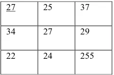
The algorithm is explained with the following steps: STEP 1: A moving or sliding window of 3 x 3 in a 512x512 image is taken.
STEP 2: The leading diagonal elements of the 3 x 3 matrix are taken and sorted.
STEP 3: The values are checked for salt and pepper noise (0 or 255) and replaced with either of the other two values which is non-noisy.
STEP 4: Shift pulse is applied to move to the next 3 x 3 sliding window.
STEP 5: The same process stated in STEP 3 is repeated for the entire image.
4.
LEADING DIAGONAL SORTING
ALGORITHM FOR RGB IMAGES
It is well known that a color image has three channels such as red, green and blue. RGB channels roughly follow the color receptors in the human eye, and are used in computer displays and image scanners. If the RGB image is 24-bit then each channel has 8 bits, in other words, the image is composed of three images (one for each channel), where each image can store discrete pixels with conventional brightness intensities varies between 0 and 255 [8,12]. The RGB image has very high resolution (48 bit) if each channel is made of 16-bit images.
The algorithm is followed for each of the three planes (RGB) STEP 1: A sliding kernel of size 3 x 3 is taken in a 512 x 512 color image
STEP 2: The leading diagonal elements of the matrix are taken and sorted.
STEP 3: The values are checked for impulse noise (0 or 255) and replaced with either of the two non-noisy values.
STEP 4: The matrix is shifted to the next 3 x 3 window. STEP 5: This process is continued for the entire image. STEP 6: This is repeated in the other two planes (step1 to step5)
STEP 7: Finally all the three planes are combined. Step 1:
Fig1: Selection of 3x3 matrix in a image
Step 2:
Fig 2: Leading diagonal elements
0 25 37 24
34 27 29 34 22 24 255 29
25 28 29 26
0 25 37
34 27 29
Step 3:
Fig3: After replacement of noisy pixel (0)
Step 4:
Fig4 : After replacement of noisy pixel (255) and final Denoised 3x3 window
5.
PERFORMANCE ANALYSIS
In order to determine the performance of various noise removal algorithms the following metric parameters are analyzed:
Peak Signal-to-Noise Ratio(PSNR)
Mean Square Error (MSE)
Structural Similarity Index Metrix
Computation Time
5.1.
Peak signal-to-noise ratio
Peak signal-to-noise ratio(PSNR) is an engineering Quantizing metric term used to assess the image reconstruction for the ratio between the maximum possible power of a signal and the power of corrupting noise that affects the fidelity of its representation. Because many signals have a very wide dynamic range, PSNR is usually expressed in terms of the logarithmic decibel scale. The PSNR is most commonly used as a measure of quality of reconstruction of lossy compression codecs (e.g., for image compression). The signal in this case is the original data, and the noise is the error introduced by compression. When comparing compression codecs it is used as an approximation to human perception of reconstruction quality, therefore in some cases one reconstruction may appear to be closer to the original than another, even though it has a lower PSNR (a higher PSNR would normally indicate that the reconstruction is of higher quality).
PSNR=10log10
=20log10
Where MAX is the maximum possible pixel value of the image.
5.2 Mean square error
The Mean Square Error (MSE) is the cumulative squared error between the compressed and the original image. MSE measures the average of the squares of the "errors." The error is the amount by which the value implied by the estimator differs from the quantity to be estimated. The difference occurs because of randomness[13,14].
MSE =
where I(i,j) is the original image, K(i,j) is the approximated version (which is actually the image which noise) and M,N are the dimensions of the images.
5.3 Structural similarity index metrix
The Structural Similarity Index Metrix (SSIM) is a effective method for measuring the similarity between two images. The SSIM index can be viewed as a quality measure of one of the images being compared provided the other image is regarded as of perfect quality. It is an improved version of the universal image quality index proposed before[13].
5.4 Computation time
Computation time or running time is the length of time required to perform a computational process. In this case, the computational process involved is the removal of noise from a noisy image.
6.
RESULTS AND DISCUSSION
[image:3.595.92.204.115.189.2]The developed algorithm is tested using 512X512 images like Lena (gray), cameraman (gray), Lena (RGB) and Zelda (RGB). The performance of the proposed algorithm is tested for all levels of noise corruption (upto 90%). Each time the test image is corrupted by salt and pepper noise of different density ranging from 10% to 90% with an increment of 10% and tested for denoising. The results obtained are hence shown in Fig.5-8. Fig.9 and Fig.10 shows the comparison graph of PSNR and MSE values respectively at different noise densities for lena(Gray) image. Fig.11 and Fig.12 gives the comparison graph of MSE and PSNR respectively at different noise densities for Lena.jpg (RGB) (512X512) image. Table 1 and 2 presents the comparison of PSNR, MSE values of different filters respectively for lena.png (512 x 512) image. Table 3 and 4 shows the comparison of MSE, PSNR values of different filters respectively for Lena.jpg(RGB) (512X512) image.
(a) (b) (c) (d)
(e) (f) (g) (h)
27 25 37
34 27 29
22 24 255
27 25 37
34 27 29
( i) ( j)
Fig.5. Results obtained for various levels of noise corrupted 512X512 lena image.(a),(c),(e),(g),(i) are the
noise corrupted lena image with noise densities 10%,30%,50%,70%,80% respectively and (b),(d),(f),(h),(j) are the corresponding restored images.
[image:4.595.57.275.140.274.2](a) (b) (c) (d)
Fig.6. Results obtained for noise corrupted 512X512 cameraman image. (a), (c) are the noise corrupted with noise densities 30% and 70% respectively and (b),(d) are
the corresponding restored images.
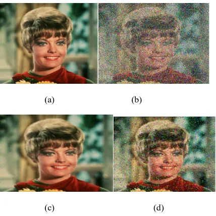
[image:4.595.306.540.212.550.2](a) (b) (c) (d)
Fig.7. Results for 50% noise corrupted Lena image(RGB) (a) original Lena image (b) 50% corrupted noise image (c) restoration result of standard median filter (d) restoration
result of proposed algorithm (LDS)
(a) (b)
(c) (d)
Fig.8. Results for 50% noise corrupted Zelda image(RGB) (a) original Zelda image (b) 50% corrupted noise image
(c) restoration result of standard median filter (d) restoration result of proposed algorithm (LDS)
The performance of the proposed algorithm is tested for various levels of noise corruption and compared with standard filters namely Median Filter (MF 3X3),Standard Median Filter (SMF) and Weighted Median Filter (WMF).The compared results are shown. In addition to the visual quality, the performance of the developed algorithm and other standard algorithms are quantitatively measured by the following parameters such as peak signal-to-noise ratio (PSNR) ,Mean square error (MSE) and Structural Similarity Index Metric ( SSIM )
Table 1.Comparison table of PSNR of different filters for lena.png (512 x 512) image
Noise density( %)
MF SMF WMF TMF Propose
d LDS 10 31.44 33.72 34.22 34.20 37.15 20 30.57 29.62 27.08 28.01 33.25 30 29.26 24.03 21.66 21.98 30.76 40 26.30 19.03 17.57 19.65 28.81 50 21.50 15.45 14.22 15.32 26.71 60 16.80 12.44 11.64 12.21 25.04 70 12.70 10.09 9.49 10.82 22.90
80 9.72 8.90 7.90 9.21 20.64
90 7.53 6.69 6.56 8.35 18.98
Fig.9.comparison graph of PSNR values at different noise densities for lena image.
Table 2.Comparison table of MSE values of different filters for lena.png (512X512) image.
Noise density
(%)
MF SMF WMF TMF Proposed
LDS
10 48.26 25.90 20.34 24.10 12.6203
20 56.95 46.10 56.25 49.01 30.95
[image:4.595.55.241.334.439.2] [image:4.595.55.269.500.714.2]Fig.10. Comparison graph of MSE values at different noise densities for lena image.
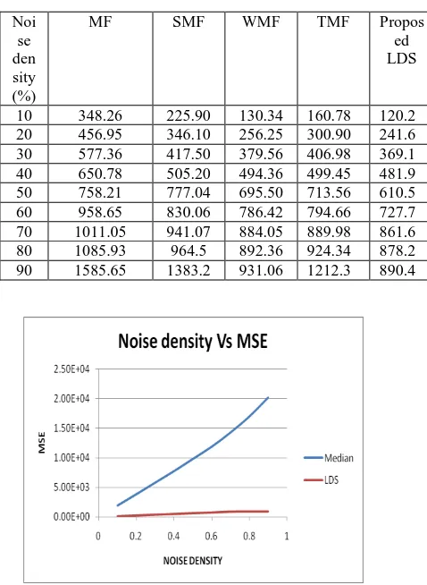
Table 3.Comparison table of MSE for Lena.jpg(RGB) (512X512) image
Noi se den sity (%)
MF SMF WMF TMF Propos
ed LDS
[image:5.595.45.284.277.604.2]10 348.26 225.90 130.34 160.78 120.2 20 456.95 346.10 256.25 300.90 241.6 30 577.36 417.50 379.56 406.98 369.1 40 650.78 505.20 494.36 499.45 481.9 50 758.21 777.04 695.50 713.56 610.5 60 958.65 830.06 786.42 794.66 727.7 70 1011.05 941.07 884.05 889.98 861.6 80 1085.93 964.5 892.36 924.34 878.2 90 1585.65 1383.2 931.06 1212.3 890.4
Fig.11. Comparison graph of MSE for Lena.jpg (RGB)
(512X512) image
Table 4.Comparison table of PSNR for Lena.jpg (RGB)(512X512) image
Fig.12. Comparison graph of PSNR for Lena.jpg (RGB)(512X512) image
Thus the plots clearly show the effectiveness of the proposed algorithm. The quantitative measures show that the LDS algorithm gives appreciable results comparatively and the visual appearance is enhanced. The Structural Similarity (SSIM) index is a method for measuring the similarity between two images. The SSIM index can be viewed as a quality measure of one of the images being compared provided the other image is regarded as of perfect quality. It is an improved version of the universal image quality index proposed and the value of SSIM to be high for better reconstructed images.
Table 5.Table showing the SSIM & Computational time for denoising lena.png
Noise density (%) SSIM Computational time (s)
10 0.9663 32.94
20 0.9262 30.93
30 0.8787 30.01
40 0.7669 29.94
50 0.6684 32.44
60 0.5219 35.41
70 0.5217 34.57
80 0.5214 32.07
90 0.5211 31.55
The above table 5 shows the various SSIM values obtained for different noise densities of Lena image and the values depict the effectiveness of the proposed LDS algorithm and also Noise
density
(%) MF SMF WMF TMF LDS
10 13.66 15.2 24.21 26.88 27.33
20 11.64 12.25 21.05 23.12 24.3
30 9.39 10.5 19.26 21.48 22.46
40 7.88 9.22 18.61 18.89 21.3
50 7.11 8.21 16.50 16.10 20.27
60 5.35 7.36 15.22 16.77 19.51
70 5.05 6.58 13.07 14.33 18.77
80 5.03 5.82 12.37 15.96 18.5
[image:5.595.341.536.595.721.2]depicts that the computational time remains constant (approx.) irrespective of the noise density for the proposed algorithm. This proves the stability of the LDS algorithm.
Thus the plots clearly show the effectiveness of proposed algorithm for 512X512 images. The quantitative measure shows that the LDS algorithm gives appreciable results comparatively. LDS algorithm works well with 512X512 image.The Comparison of the various Sorting Techniques is shown in Table 6 and proves the effectiveness that LDS requires only three comparisons.
Table 6.Comparison of the various Sorting Techniques
The illustration of LDS algorithm is shown in the table 6 containing the comparison of the various sorting techniques. It is observed that only 3 comparisons are required to compute a median 3x3 window, thus resulting in a drastic improvement of computational complexity and hence the computational time required for denoising the image [5,14].
7.
CONCLUSION
An efficient non-linear algorithm to remove salt and pepper noise in Gray scale and RGB image is proposed. The Lone Diagonal Sorting algorithm clearly reduces the computational time required for denoising the corrupted images. Also since the noisy pixels are replaced with the neighborhood pixels, the image quality is comparatively appreciable. The lower number of computations performed obviously reduces the hardware complexity, thereby increasing the efficiency and reducing the cost of the system compared to the other competitive algorithms appreciable. The lower number of computations performed obviously reduces the hardware complexity and thereby increasing the efficiency and reducing the cost of the system compared to the other competitive algorithms. The work could be extended by using non local approach along with LDS algorithm [10,12].
8.
REFERENCES
[1] Rafael C. Gonzalez, Richard Eugene Woods, Steven L.Eddins .2004.Digital image Processing. Pearson Education.
[2] Jayaraman,S., Veerakumar,T., and Esakkirajan,S. 2009.Digital Image Processing.Tata McGraw-Hill Education.
[3] Gallagher, N.C.,Jr. and Wise,G.L.1981.A Theoretical Analysis of the Properties of Median Filters. IEEE Trans. Acoust., Speech and Signal Processing, 29, 1136-1141. [4] Nodes,T.A,,Gallagher,N.C. 1987.Median Filters: Some
Modifications and their properties.IEEE Trans. Acoust., Speech and Signal Processing, 30, 739-746 .
[5] Astola,J.,Kuosmanen.P. 1997.Fundamentals of Non-Linear Digital Filtering. BocRaton, CRC.Forman, G. 2003. An extensive empirical study of feature selection metrics for text classification. J. Mach. Learn. Res. 3 (Mar. 2003), 1289-1305.
[6] Yin,L.,Gabbouj,M., and Neuvo,Y.1996.Weighted Median Filters: A Tutorial.IEEE Transactions on Circuit and and Systems - 11: Analog and Signal Processing, 4(3).
[7] Brownrig,D.R.1986.Generation of Representative members of a Weighted median filter class. Proc. Inst. Elec. Eng. (133), 445-448.
[8] Chen, L.,Chiueh,T.D and Hsiao,J.1994.Design and VLSI Implementation of Real-Time Weighted Median Filters.Proc. 1994 Asia-Pacific Conference on Circuit and Systems, 91-96.
[9] Chan,R.H.,Ho,C.W., and Nikolova,M.2005.Salt and pepper noise removal by median type noise detectors and detail reserving regularization.IEEE Transactions on Image Processing,14(10), 1479-1485.
[10]Buades.,Coll, A.B., and.Moral,J.M.2005.A Review of image denoising algorithms with a new one.Multiscale model.simul.,4(2), 490-530.
[11]Esakkirajan,S.,Veerakumar,T., Adabala Subramanyam, N.,and PremChand,C.H.2011.Removal of High Density Salt and Pepper Noise Through Modified Decision based.Unsymmetric Trimmed Median Filter. IEEE signal processing letters,18(5), 287-291
[12]Vijaykumar,V.R.,Ebenezer,D.,and Vanathi ,P.T.2008.Detail preserving median based filter for impulse noise removal in digital images, IndiaICSP2008 Proceedings IEEE, 978-1-4244-2179-4.
[13]Fang et al.,2004.Speckle Noise Reduction in SAR Imagery Using a Local Adaptive Median Filter”, GIScience and Remote Sensing, 41(3), 244-266.
[14]Subhojit Sarker, Shalini Chowdhury, Samanwita Laha and Debika Dey.2012.Use of non-local means filter to denoise image corrupted by salt and pepper noise,Signal & Image Processing : An International Journal”, 3(2), DOI : 10.5121/sipij.2012.3217 223.
Sorting Techniques
No. of comparisons to compute median
Bubble
Sort 36
Shear sort 18
Lone diagonal sort