Are analysts' loss functions asymmetric?

Lancaster University Management School

Working Paper

2005/071

Are analysts' loss functions asymmetric?

Mark Clatworthy, David Peel and Peter Pope

The Department of Economics

Lancaster University Management School

Lancaster LA1 4YX

UK

© Mark Clatworthy, David Peel and Peter Pope All rights reserved. Short sections of text, not to exceed two paragraphs, may be quoted without explicit permission,

provided that full acknowledgement is given.

Are Analysts’ Loss Functions Asymmetric?

M. A. Clatworthy, D.A. Peel and P.F. Pope

*

Are Analysts’ Loss Functions Asymmetric?

1. Introduction

Financial analysts’ forecasts of corporate earnings are an important input to investors’ decision models,

e.g. valuation models. Yet there is extensive evidence suggesting that analysts’ forecasts are “irrational” –

specifically they appear to be biased (ex post forecast errors have a non-zero mean) and inefficient (ex

post forecast errors are correlated with information known at the forecast date).1 _{Recent work has}

proposed two explanations for such findings based on the idea that the statistical bias and inefficiency of

forecasts is rational and originates in the loss functions underpinning analysts’ forecast decisions, i.e. how

analysts weight prospective prediction errors when deciding on “optimal” earnings forecasts. For example,

Gu and Wu (2003) and Basu and Markov (2004) suggest that analysts have linear loss functions. A

mutually exclusive alternative explanation is that analysts have asymmetric loss functions, perhaps

motivated by private incentives originating in business relationships between securities firms and their

investment banking clients, or in analysts’ dependence on managers for information (e.g. Lin and

McNichols, 1998; Dugar and Nathan, 1995; Lim, 2001; Hong and Kubik, 2003).2 _{Prior research reports}

evidence consistent with both explanations, but does not test the linear loss explanation against the

asymmetric loss alternative. Better understanding of the nature of analysts’ loss functions is potentially

important for investors. Although it is investors’ loss functions which ultimately determine investment

decisions, interpretation and use of analysts’ forecasts by investors should reflect beliefs concerning

analysts’ loss functions (Lambert, 2004, p.221). This paper contains new evidence suggesting analysts’

earnings forecasts are driven by asymmetric loss functions.

1 _{See Kothari (2001) for a review.}

2 _{Other explanations forecast bias and inefficiency proposed in the literature suggest either that analysts are irrational}

Understanding the nature of analysts’ loss functions is relevant to interpreting and using forecasts

because a rational analyst’s “optimal” earnings forecast depends on both the subjective probability

distribution of earnings and on the analyst’s loss function. A rational analyst with a quadratic loss function

minimizes the mean squared value of anticipated forecast errors (MSE), and in this case the optimal

forecast is the conditional mean of earnings and the expected value of the mean forecast error is zero;

however, the median forecast error depends on the distribution of earnings. In contrast, a rational analyst

with a symmetric linear loss function minimizes the mean absolute value of anticipated forecast errors

(MAE), the optimal forecast is the conditional median and the expected value of the median forecast error

is zero, while the mean value depends on the distribution of earnings. Similar to a quadratic loss function,

a linear loss function is symmetric in weighting positive and negative forecast errors of the same

magnitude, but it gives less weight to extreme forecast errors.3 _{In the case of asymmetric loss functions,}

optimal forecasts are not consistent with the MSE or MAE criteria and both mean and median forecast

errors can have expected values different from zero (Keane and Runkle, 1998). The properties of forecast

errors under asymmetric loss depend on both the distribution of earnings and on the functional form and

parameters of the loss function.

We test whether analysts produce forecasts consistent with asymmetric loss functions against the

alternative of symmetric loss (either quadratic or linear). Our analysis is based on theoretical predictions

relating forecast errors to the variance and skewness of the forecast error distribution. Our approach builds

on Gu and Wu (2003), who conjecture that, due to analysts facing linear loss functions, the magnitude of

forecast errors depends on ex ante skewness of the earnings (and hence of forecast error) distribution,

though not on the variance. Consistent with this prediction, Gu and Wu (2003) report evidence that

forecast errors are positively associated with the skewness of earnings, although they do not control for

variance. Our analysis of asymmetric loss assumes that analysts’ loss functions belong to the Linex class

of asymmetric loss functions introduced by Varian (1974) and Zellner (1986). Under Linex loss functions,

3 _{Granger (1969) proposes a piecewise linear (LIN-LIN) loss function that weights positive and negative forecast}

forecast errors are predicted to depend on the variance of the forecast error. If the distribution of forecast

errors is conditionally non-normal, forecast errors under Linex loss functions also depend on higher

moments, including skewness. The linear (MAE) loss function is a special limiting case in which forecast

errors depend only on skewness. Dependence of forecast errors on the forecast error variance under

Linex-class asymmetric loss functions but not under linear loss functions suggests a way of discriminating

between symmetric linear and asymmetric loss functions.

We test whether the ex ante variance of the forecast error is incrementally significant in a

regression that includes both variance and skewness instruments. Our results confirm that the ex ante

forecast error variance instrument is a significant determinant of the forecast error. This is consistent with

financial analysts having asymmetric loss functions. Further analysis reveals that the dominant role of

forecast error variance in explaining forecast bias is robust across portfolios formed on the basis of

book-to-price ratio and market capitalization. These firm characteristics are known determinants of forecast

error accuracy and skewness.

The rest of the paper is organized as follows. In section 2, we discuss the theory of the Linex loss

function and derive empirical predictions that distinguish between linear and asymmetric loss. In section 3

we describe our empirical research design. In section 4 we describe our dataset and report our empirical

results. Section 5 contains our conclusions.

2. Loss functions and forecast bias

Two elements of the forecasting process determine whether a rational earnings forecast is biased.

The analyst’s loss function and the subjective probability distribution associated with the variable being

forecasted combine to generate an optimal forecast. If the subjective probability distribution of earnings is

skewed, rational forecasts produced by analysts with symmetric loss functions will be biased, unless the

loss function is quadratic (Gu and Wu, 2003; Basu and Markov, 2004). However, earnings skewness is not

necessary for optimal forecasts to be biased because of the role played by the loss function. Although

developed for general asymmetric loss functions, the properties of optimal forecasts have been analyzed

for two specific asymmetric loss functions: Lin-Lin and Linex.

Granger (1969) demonstrates that even if the data generating process for a variable follows an

unconditional Gaussian process, optimal forecasts will exhibit constant bias when the forecaster optimizes

with reference to an asymmetric, piecewise-linear, Lin-Lin loss function. In this case the constant

marginal loss (or cost) associated a unit forecast error above some threshold (e.g. zero) is different from

the constant marginal loss for a unit forecast error below the threshold. The magnitude of the optimal bias

depends on the parameters of the loss function, and on the forecast error variance. Christofferson and

Diebold (1996, 1997) extend Granger’s analysis to conditional Gaussian processes. In this case, optimal

forecasts exhibit time-varying bias, conditional on the time-varying forecast error variance.

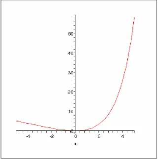
The Linex loss function is a more general asymmetric loss function specification than Lin-Lin

(Varian, 1974; Zellner, 1986). Assume that the variable to be forecast is earnings at time t, denoted yt. The

Linex loss function has the form:

2

(

1)

t

x t

e

ax

L

α

α

−

−

=

(1)

where

α

is a constant and xtis the forecast error at time t, defined as

x

t

≡

y

t

-

f

t, where

f

t is the forecast.

The parameter

α

determines the degree of asymmetry. A Linex function with

α

= 0.7 is plotted in Figure

1. A convenient property of the Linex loss function is that it nests the quadratic loss function asα→0.4

Under the Linex loss function, optimistic forecasts (negative forecast errors) are more costly than

pessimistic forecasts (positive forecast errors) when

α

< 0. In this case, the loss is approximately

exponential in x if x < 0, and approximately linear in x if x > 0. Conversely, if

α

> 0, the Linex function

is exponential to the right of the origin, and linear to the left. In this case, pessimistic forecasts (positive

forecast errors) are more costly than optimistic forecasts (negative forecast errors).

4 _{As α→ 0, the numerator and the denominator of (1) tend to zero. Consequently, as α→ 0, we employ L’Hospital’s}

Assume initially earnings, yt, are generated by a conditional Gaussian process. Diebold and

Christofferson (1996, 1997) show that under the Linex loss function (1), the optimal h-period ahead

forecast, ft,t+h,is given by:

f

_{t t h,+}

=

E

_t

(

µ

_{t h+}

)

+

α

E

_t

(

σ

_{t h t+}

)

2

2 ₍₂₎

where E_t(µ_{t h+} ) is the expectation of the mean of yt+h conditional on information at time t (and is the

optimal forecast under quadratic loss) and is the expectation of the conditional error variance

over the h periods. Expression (2) tells us that the optimal forecast for a rational analyst with an

asymmetric loss function, given by the Linex function (1), differs from the conditional mean, i.e. the

forecast is biased. It is optimal for the analyst to produce optimistic forecasts if

E

_t

(

σ

_{t h}2₊

₎

α

> 0. Diebold and

Christofferson (1996, 1997) also show that the ex post forecast error,

x

_t, is given by:

2

(

)

2

t t t h t

x

= −

α

E

σ

₊

+

z

(3)

where is a zero mean moving average error process of order

z

_t h- 1.

Expressions (2) and (3) indicate that the optimal bias for an asymmetric loss analyst depends

positively on the loss function parameter,

α

, and on the variance of the forecast error. Thus, given that the

forecast error variance, , is positive, if forecast errors are on average negative (forecasts are on

average optimistic), this is consistent with a positive loss function parameter,

E

_t

(

σ

_{t h}2₊

₎

α

.

The optimal forecast expression (2) assumes that the outcome (earnings) series, yt,, is a conditional

Gaussian process. If we relax this assumption, it is possible to show that the optimal forecast and the

forecast error depend on both the variance and the skewness of the forecast error process. The forecast

error is given by:

2 3

[ (

), (

)]

t

t t t h t t h

where is a moving average error process, is the expectation of conditional skewness in the

forecast error and G is a nonlinear, positive function of both the conditional variance and the conditional

skewness of the forecast error process (see Appendix A for the proof). *

t

z

E

_t

(

σ

_{t h}3₊

₎

Expressions (3) and (4) have important empirical implications, given that the distributions of

earnings and earnings forecast errors are non-normal (e.g. Gu and Wu, 2003; Abarbanell and Lehavy,

2003). Under asymmetric loss, if

α

> 0 then forecast bias is expected to depend on the positively on the

variance of the forecast error. The theory also predicts that forecast errors will be positively related to

skewness, although the association will be weak if the magnitude of

α

is small. In contrast, if the loss

function is linear and symmetric (MAE), as assumed by Gu and Wu (2003), forecast bias depends only on

the skewness of earnings (or forecast errors). This suggests that a simple test of whether analysts’ loss

functions are asymmetric is to examine dependence between forecast errors and the proxies for the

conditional variance and conditional skewness of forecast errors. If only skewness is significant then this

is consistent with analysts minimising absolute forecast errors. If variance of forecast error is a significant

determinant of forecast errors then the hypothesis that analysts minimize absolute forecast error can be

rejected in favour of an asymmetric loss function, under the maintained assumption of rational

expectations.

3. Research design

We assume that analysts’ loss functions take account of any scale-related component of forecast errors.

Since analysts forecast earnings per share, the magnitude of raw forecast errors will depend on the “scale”

of the stock. Holding the size of firms constant, a firm with N issued shares will have earnings per share

forecast errors that are twice as large as an otherwise identical firm with 2N issuedshares. If we assume

that costs associated with forecast errors are related to the proportionate valuation errors that could arise

error.5 _{However, while our main tests employ price-scaled forecast errors, in unreported sensitivity checks}

we also estimated regressions using un-scaled data. In this case, we scale ERROR and the prior periods’

earnings change variables (SUE1 and SUE2) by stock price at t-1. Our tests are based on the empirical

model in Gu and Wu (2003).6 _{We extend their model by adding a proxy for the conditional variance and}

skewness of forecast errors. The main estimating equation is as follows:

it it it it it it it it it SUE b SUE b LOSS b ANFLL b MVAL b ERRSKEW ERRVAR b ERROR ε λ λ + + + + + + + + = 2 1 ln ln 5 4 3 2 1 2 1

0 ₍₅₎

In line with Gu and Wu (2003), ERROR is defined as actual quarterly earnings taken from I/B/E/S minus

the median of all forecasts of quarterly earnings issued within 90 days of the earnings announcement,

scaled by beginning-of-period stock price. ERRVAR is defined as the second moment of the previous 8

quarters’ scaled forecast errors for firm i, while ERRSKEW is the third moment of the previous 8 quarters’

scaled forecast errors for firm i. lnMVAL is the natural logarithm of market value at the beginning of

quarter t and is included to control for the possibility that analysts issue more biased forecasts for smaller

companies in order to obtain access to management where less information is available (Francis and

Willis, 2001). lnANFLL is the natural log of the number of analysts issuing forecasts for firm i in quarter t

(Gu and Wu, 2003). We also include LOSS as an indicator variable (equal to 1 if the consensus forecast of

earnings is negative, zero otherwise) because it has been argued that forecasts of losses are more

optimistic (e.g. Duru and Reeb, 2002). SUE1and SUE2 are included to control for analyst underreaction

(e.g. Abarbanell and Bernard, 1992) and are defined as, respectively, the one period and two period lagged

earnings surprise based on a seasonal random walk model.

5 _{For example, suppose that intrinsic value is estimated using the P/E multiple approach and is a multiple of forecast}

earnings per share. Then the per share intrinsic value estimation error is proportional to the scaled forecast error.

6 _{Although Gu and Wu’s (2003) model forms the basis for our tests, there are differences between our model and}

theirs. For instance, they include measures of earnings variability and forecast variability as control variables in their test of the MAE loss function, whereas we include the variance of the forecast error as a central test of an

asymmetric loss function. We note that theoretically it is the moments of forecast errors that are relevant

4. Empirical tests

4.1 Data

Our sample is drawn from the I/B/E/S detail history files for the period 1983 to 2003. To ensure

consistency, we retrieve individual quarterly forecasts, actual earnings, earnings announcement dates and

stock price data all from I/B/E/S. We require each firm to have at least eight consecutive quarters’ actual

earnings and forecast data in order to generate our measures of forecast error variance and skewness. We

define the consensus forecast as the median of all forecasts issued within 90 days of the earnings

announcement date. Forecast error (ERROR)is defined as actual earnings at time t, minus the consensus

forecast, divided by stock price at the beginning of the forecast period, multiplied by 100. Negative errors

therefore imply analyst optimism.

We measure error variance as the unstandardised variance of ERROR in the preceding eight

periods, i.e., the sum of the squared deviations from the mean of ERROR over the previous eight quarters.

Our measure of skewness is defined as the sum of the cubed deviations from the mean ERROR for the

eight quarters prior to quarter t. In order to remove potential data errors, we winsorize the error and

earnings related variables at the 1st _{and 99}th _{percentiles, in line with previous research (Abarbanell and}

Lehavy, 2003). Our results are robust to alternative outlier deletion procedures (e.g. removing

observations in the 5th _{and 95}th _{percentiles).}

4.2 Descriptive statistics

Our final sample comprises 79,653 firm quarters for 4,335 firms. Table 1, panel A, provides summary

statistics. In line with prior research (e.g. Basu and Markov 2004), the sample-wide distribution of forecast

error is negatively skewed, with the mean forecast error being negative (consistent with on-average

optimism bias) and the median forecast error being slightly positive. Our measures of firm-specific ex ante

error variance (ERRVAR) and skewness (ERRSKEW) both display a high degree of variability. The

make a loss and the median number of analysts following each firm in quarter t is 6. Panel B provides

reassurance that the forecast error distribution in our sample is consistent with the prior literature by

comparing our sample with that in Abarbanell and Lehavy (2003). The comparison shows that the two

samples are very similar, despite the forecast data being from different data sources.

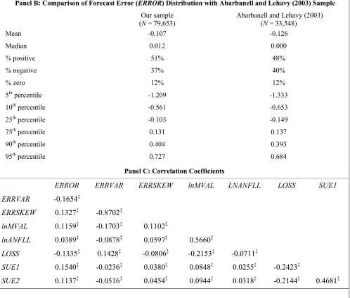
Panel C of table 1 reports the correlations between variables. Particularly noteworthy is the high

negative correlation between ERRVAR and ERRSKEW. This suggests the possibility that skewness could

be serving a proxy role for variance in Gu and Wu (2003). Since dependence of the forecast error on

variance is key empirical prediction that distinguishes the symmetric (linear) loss explanation of forecast

bias from the asymmetric loss explanation, this characteristic of the data points to the importance of

controlling for variance in evaluating these two competing explanations.

4.3 Regression results

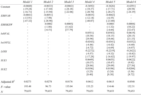
Our main regression results are reported in Table 2. We estimate six versions of equation (5) including

one or both of ERRVAR and ERRSKEW and both with and without control variables. In view of the clear

non-normality in the distribution of forecast errors in table 1, the possibility exists that inferences are

sensitive to heteroskedasticity and non-normality in regression errors. Therefore we report both OLS t –

statistics (as in Gu and Wu, 2003) and t –statistics based on White robust standard errors.7 _{Table 2}

indicates that the White corrected t-statisticsare often very much lower than the OLS t-statistics, and

inferences regarding the significance of ERRSKEW are sensitive to the choice of test statistic.

Breusch-Pagan (1979) tests rejected the null of constant variance in all reported models. We therefore rely on the

more conservative White corrected t-statistics, where relevant.

7 _{We also examined the sensitivity of inferences to use of exact critical values for the White standard errors obtained}

from the Wild bootstrap methodology. Although critical values obtained from the bootstrap methodology are much higher than classical values, indicating that non-normality is a significant problem, the main inferences are

The results in table 2 generally confirm prior research. Models 3 and 6 reveal a significant positive

association between ERROR and ERRSKEW when ERRVAR is excluded.8 _{This is consistent with Gu and}

Wu (2003). Results for models 1 and 4 indicate that if ERRSKEW is replaced by ERRVAR, model

specification improves (adjusted R2 _{increases from 1.76% (5.48%) without (with) control variables to}

2.73% (6.12%)). The sign of the coefficients on ERRVAR are negative, as predicted if positive forecast

errors are more costly to analysts than negative forecast errors, i.e. if α > 0. Results for models 2 and 5

indicate that the statistical significance of ERRVAR remains, even after controlling for ERRSKEW, and

despite the high correlation between ERRVAR and ERRSKEW that would be expected to bias t-statistics

towards zero.9 _{Note, however, that when ERRVAR isincluded in the model,the sign of the coefficient on}

ERRSKEW in models 2 and 5 is negative, as predicted by the asymmetric loss function explanation of

forecast bias, and in contrast to the positive coefficients in models 3 and 6. Further, based on White

corrected t-statistics, the significance of ERRSKEW is at best marginal, whereas using OLS t-statistics

ERRSKEW appears highly significant.

Generally the results in table 2 indicate that results are not sensitive to inclusion of control

variables. Inferences regarding the significance of ERRVAR and ERRSKEW are identical for model 1-3

and for models 4-6. Therefore, in subsequent tests we focus on models 1-3. The estimated parameters for

the control variables in models 4-6 are generally in line with the findings in prior research. Forecast errors

are positively related to firm size (as captured by lnMVAL) in each of the reported models, suggesting that

analysts are more optimistic when forecasting earnings of smaller firms. We further examine this issue

below. There are significant negative coefficients on the analyst following variable (lnANFLL) and the

loss variable (FCLOSS), both of which are consistent with Gu and Wu (2003). Like many previous

studies (e.g., Abarbanell and Bernard, 1992; Easterwood and Nutt, 1999), there is also evidence of

8 _{Gu and Wu (2003) employ measures of variance and skewness based on the distribution of earnings. We use}

measures based on the distribution of forecast errors, to be consistent with theory. However, empirically, measures under the two approaches are highly correlated. If we replace our measures with measures similar to Gu and Wu (2003) we obtain qualitatively similar results to those reported here. Details are available from the authors.

9 _{Despite the high univariate correlation between ERRVAR and ERRSKEW, all variance inflation factors in the}

underreaction to prior period earnings changes – coefficients on both SUE1 and SUE2 are significant and

positive in each of models 4-6.

Overall, we interpret the results in table 2 as providing strong support for the conjecture that

analyst forecast bias is associated with analysts having asymmetric loss functions, rather than linear

symmetric loss functions. If analysts’ loss functions are linear and symmetric, forecast errors should be a

function of ERRSKEW but not ERRVAR, whereas asymmetric loss should result in the statistical

significance of ERRVAR, with ERRSKEW having the same sign as ERRVAR. This is exactly what we find

in our results.

4.4 Book-to-market and size portfolio analysis

The results reported in table 2 are based on a very large sample and unreported analysis reveals they are

extremely robust to various model specification and variable measurement choices (see section 4.5

below). In this section we show that the findings reported above extend to portfolios sorted on a priori

determinants of analyst forecast bias that are also correlates of forecast error variance and skewness. We

consider the relation between forecast errors and ERRVAR and ERSKEW for portfolios sorted on the basis

of book-to-market ratio and on market capitalization. If ERRVAR retains it ability to explain

within-portfolio forecast errors, this constitutes an even more powerful test of the asymmetric loss function

explanation.

We sort portfolios on the basis of these stock characteristics first because they are the basis of

commonly used investment styles - book-to-market ratio is a common characteristic for distinguishing

between value and glamour stocks. Doukas et al. (2002) show that analyst forecast bias differs

significantly across portfolios sorted on these characteristics, although not in a direction capable of

explaining the value premium the irrational extrapolation hypothesis. Second, recent research suggests

and Ryan, 2005) and, that conservatism is an important determinant of the distributional properties of

earnings and forecast errors (see, e.g., Basu, 1997; Helbok and Walker, 2004).

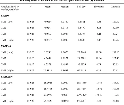
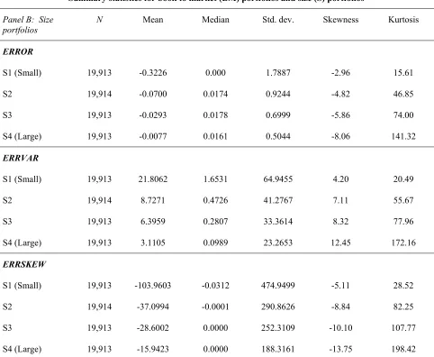
We form one-way sorted portfolios each quarter based on beginning-of-quarter book-to-price and

on market capitalization. Table 3 confirms that forecast errors are indeed dramatically different across

book-to-market ratio and market capitalization portfolios. The mean values of ERROR lie between

-0.01% for low book-to-market stocks to -0.28% for high book-to-market stocks, indicating that the

optimistic bias is much higher for high book-to-market stocks. Note also that the standard deviation of

ERROR increases and the negative skewness decreases monotonically across book-to-market portfolios. In

contrast the stock level estimates of ERRVAR and ERRSKEW indicate that forecast error variance

increases dramatically with book-to-market and forecast error skewness is negative and decreases

dramatically with book-to-market. Similar patterns are observed across size-sorted portfolios. The degree

of optimistic bias in forecasts is much higher for small firms, and ERRVAR decreases dramatically as

firms become larger, as does the extent to which ERRSKEW is negative. The patterns of ERRVAR and

ERRSKEW across characteristic portfolios are consistent with the observed forecast error bias.

In Table 4 we estimate models 1-3 similar to table 2, but for the one-way sorted portfolios. Results

are generally consistent with table 2.10 _{Panel A reports results for portfolios sorted on book-to-market. The}

coefficient on ERRVAR when it is the sole independent variable is consistently negative, as predicted by

the asymmetric loss function explanation, and significant at the 10% level or better. Similarly, the

coefficient on ERRVAR in model 3 is positive and significant in three out of four cases. When both

ERRVAR and ERRSKEW are included in the same regression (model 2), multi-collinearity problems

become somewhat more severe but ERRVAR retains its significance for high book-to-market portfolios

where forecast bias is greatest. The sign on ERRSKEW changes from positive to negative in three out of

four cases, although it is significant in only one case.

10 _{Additional (unreported) tests showed that the results in table 4 are not sensitive to the inclusion of the control}

Results in table 4 panel B for size-sorted portfolios are similar. ERRVAR is negative and

significant for all portfolios in model 1, while ERRSKEW is positive and significant. When ERRVAR and

ERRSKEW are entered jointly, only ERRVAR is significant (in three cases at better than the 10% level) .

ERRSKEW is insignificant in all cases. Again, multi-collinearity does present a problem for some

portfolios, especially in the case of the larger firm portfolios, and this explains why ERRVAR loses

significance when ERRSKEW is added.

Overall, the results in table 4 confirm that the variance of forecast errors is a significant

determinant of forecast bias, even after first sorting firms into portfolios based on stock characteristics that

sharply discriminate between different levels of forecast bias and forecast error variance and skewness.

The continued significance of ERRVAR as an explanatory factor for forecast errors supports the earlier

evidence in favour of the conjecture that financial analysts form their forecasts with reference to

asymmetric loss functions.

4.5 Robustness checks

The results we have reported are based on price-scaled forecast errors. We believe that there are

good reasons for scaling, based on considering the links between forecast errors and the costs borne by

users of earnings forecasts (see e.g. footnote 5). However, there is accumulating evidence that scaling may

have perverse effects on the distributional properties of variables (see, e.g., Cohen and Lys, 2003;

Durtschi and Easton, 2004; Lambert, 2004). For this reason, we also employed the Wild bootstrap

methodology to both price-scaled and un-scaled data and identified critical values for relevant test

statistics (e.g. Davidson and Flachaire, 2001). This methodology utilizes the distribution of the error term

in the main estimating equation to simulate empirical confidence intervals necessary to reject the null

hypothesis when the null holds. It provides a powerful test of statistical significance when the underlying

regression error distribution is non-normal (Wu, 1986; Hardle and Mammen, 1993). Use of the Wild

to our estimates, critical values to allow rejection of the hypothesis that skewness is significantly different

from zero are up to 74% higher than the classical value (for p< 0.05) for un-scaled data. Despite this, in

unreported results we find that all the inferences drawn from the main results reported in table 2 remain

intact, after taking account of the bootstrapped critical values.

As a further robustness check, we also estimated Models 1–6 using least absolute deviation (LAD)

regression, as used by Basu and Markov (2004) and Fama MacBeth (1973) regressions. The results (not

reported) are again consistent with those reported in Tables 2 and 4.

5. Conclusions

Previous research has consistently found evidence of bias and inefficiency in financial analysts’ forecasts

of earnings. Recent research by Gu and Wu (2003) and Basu and Markov (2004) has examined the

possibility that these findings are attributable to an unrealistic assumption of a quadratic loss function, and

has concluded that analysts’ objective is to minimise the mean absolute forecast error (MAE), rather than

mean squared error. The mean absolute error loss function penalises forecast optimism and pessimism

equally. The explanation for forecast bias is attributable to skewness in the distribution of earnings.

However, numerous studies suggest that analysts’ motives may be driven by the costs associated with

under-predicting earnings being higher than the costs of over-predicting earnings, i.e. asymmetric loss

functions. Asymmetric loss functions could result from incentives to gain access to management and/or

more favourable career prospects for analysts who are systematically optimistic (e.g., Lim, 2001; Hong

and Kubik, 2003). In this paper, we test whether analysts’ forecasts are consistent with loss functions

being asymmetric.

Under the MAE loss function, forecast error is a function only of forecast error skewness. In

results indicate that the linear symmetric loss function of MAE can be rejected in favour of the Linex

function. We find that forecast error is more strongly related to prior forecast error variance than to

skewness. Indeed, when forecast error variance is included in forecast error regressions, the sign on

forecast error skewness changes. These results strongly suggest that analysts have asymmetric loss

functions.

Our results have important implications for the interpretation of analysts’ forecasts. The

assumption that analysts’ objective is solely to minimise forecast error may be inappropriate. As pointed

out by Lambert (2004), it is investors’, rather than analysts’, loss functions that are ultimately most

important in determining security prices. However, to the extent that analysts’ forecasts influence

investors’ decision making, an understanding of the shape of analysts’ loss function is necessary to enable

References

Abarbanell, J. and R. Lehavy (2003). ‘Biased forecasts or biased earnings? The role of reported earnings in explaining apparent bias and over/underreaction in analysts’ earnings forecasts.’ Journal of Accounting and Economics, 36: 105-146.

Basu, S. (1997). ‘The conservatism principle and the asymmetric timeliness of earnings.’ Journal of Accounting and Economics, 24: 3-37.

Basu, S. and S. Markov (2004). ‘Loss function assumptions in rational expectations tests on financial analysts’ earnings forecasts.’ Journal of Accounting and Economics, 38: 171-203.

Beaver and Ryan (2005). ‘Conditional and unconditional conservatism: concepts and modelling.’ Review of Accounting Studies, forthcoming.

Breusch, T. and A. Pagan (1979). ‘A simple test for heteroskedasticity and random coefficient variation.’

Econometrica, 47: 1287-1294.

Chatterjee, S. and B. Price (1977). Regression Analysis by Example, New York: John Wiley & Sons.

Christofferson, P.F. and F. Diebold (1996). ‘Further results on forecasting and model selection under asymmetric loss.’ Journal of Applied Econometrics, 11: 561-572.

Christofferson, P.F. and F. Diebold (1997). ‘Optimal prediction under asymmetric loss.’ Econometric Theory, 13: 808-817.

Cohen, D.A. and T.Z. Lys (2003). ‘A note on analysts’ earnings forecast errors distribution.’ Journal of Accounting and Economics, 36: 147-164.

Das, S., C. Levine and K. Sivaramakrishnan (1998). ‘Earnings predictability and bias in analysts’ forecasts.’ The Accounting Review, 73: 277-294.

Doukas, J.A., C.F. Kim, and C. Pantzalis (2002). ‘A test of the errors-in-expectations explanation of the value/glamour stock returns performance: evidence from analysts’ forecasts.’ Journal of Finance, 57(5): 2143-2165.

Dugar, A. and S. Nathan (1995). ‘The effect of investment banking relationships on financial analysts’ earnings forecasts and investment recommendations.’ Contemporary Accounting Research, 12(1): 131-160.

Durtschi, C. and P. Easton, (2005). ‘Earnings management? The shapes of the frequency distributions of earnings metrics are not evidence ipso facto.’ Journal of Accounting Research, 43(4): 557-592.

Duru, A. and D.M. Reeb (2002). ‘International diversification and analysts’ forecast accuracy and bias.’

The Accounting Review, 77: 415-433.

Easterwood, J.C. and S.R. Nutt (1999). ‘Inefficiency in analysts’ earnings forecasts: systematic misreaction or systematic optimism?’ Journal of Finance, 54(5): 1777-1797.

Fama, E.F. and J.D. MacBeth (1973). ‘Risk, return, and equilibrium: empirical tests.’ Journal of Political Economy, 80(3):607-636.

Francis, J. and R.H. Willis (2001). ‘An alternative test for self-selection in analysts’ forecasts.’ Duke University working paper.

Friesen, G. and P.A. Weller (2002). ‘Quantifying cognitive biases in analyst earnings forecasts.’ Working paper, University of Iowa.

Granger, C.W.J. (1969).‘Prediction with a generalised cost of error function.’ Operational Research Quarterly, 20: 199-207.

Gu, Z. and J.S. Wu (2003). ‘Earnings skewness and analyst forecast bias.’ Journal of Accounting and Economics, 35: 2-29.

Helbok, G. and M. Walker (2004). ‘On the nature and rationality of analysts’ forecasts under earnings conservatism.’ British Accounting Review, 36:45-77.

Hong, H. and J.D. Kubik (2003). ‘Analyzing the analysts: career concerns and biased earnings forecasts.’

Journal of Finance, 58(1): 313-351.

Kang, S., J. O’Brien and K. Sivaramakrishnan (1994). ‘Analysts’ interim earnings forecasts: evidence on the forecasting process.’ Journal of Accounting Research, 32(1): 103-113.

Keane, M.P. and D.E. Runkle (1998). ‘Are financial analysts’ forecasts of corporate profits rational?’

Journal of Political Economy, 106(4): 768-805.

Kothari, S.P. (2001). ‘Capital Markets Research in Accounting.’ Journal of Accounting and Economics,

31: 105-231.

Lambert, R.A. (2004). ‘Discussion of analysts’ treatment of non-recurring items in street earnings and loss function assumptions in rational expectations tests on financial analysts’ earnings forecasts.’ Journal of Accounting and Economics, 38: 205-222.

Lim, T. (2001). ‘Rationality and analysts’ forecast bias.’ Journal of Finance, 56(1): 369-385.

Lin, H. and M. McNichols (1998). ‘Underwriting relationships, analysts’ earnings forecasts and investment recommendations.’ Journal of Accounting and Economics, 25: 101-127.

McNichols, M. and O’Brien, P. (1997). ‘Self-selection and analyst coverage.’ Journal of Accounting Research, 35 (supp): 167-199.

Varian, H. (1974). ‘A Bayesian approach to real estate assessment,’ in S. E. Feinberg and A. Zellner (eds.), Studies in Bayesian Economics in Honour of L. J. Savage. Amsterdam: North Holland: 195-208.

Appendix A

Expanding the Linex function (1) to a fourth-order Taylor approximation we obtain

2 3 2 4

2

(

1)

+

+

2

6

24

t

x t

e

ax

x

x

x

L

α

_α

_α

α

−

−

=

≅

(A1)

Noting that x y≡ − f and minimising L with respect to the forecast, we obtain

2 2 3

0

2 6

dL x x

x df

α α

= + + = (A2)

Taking expectations of (A2) we obtain the cubic equation:

2 2 3

[

2 6

x x

E x+α +α ] 0=

2

3 )

(A3)

Let Z = E(y) – f and y - E(y) = ε. Noting that

2 2

3 3

( ) ( ) and

( ) (

x y Ey Ey f y Ey Z

x y Ey Ey f y Ey Z

= − + − = − +

= − + − = − +

we obtain

2

2 2 3 2 3

( ) ( 3 )

2 6

Z ε Z ε εZ Z

α _σ α _{σ σ}

+ + + + + =0

3

(A4)

3 3

where ( )σ_ε =E ε =E y E y( − ( )) .

Rearranging (A4) we obtain equation (4) in text.

Note that if we approximate (A1) to order 3 we obtain

₍ 2 2₎

2 ε

α σ

+ + =0

Z Z .

Therefore

2 2

2 2

Z+αZ = −α σ_ε.

If α > 0 then Z becomes more negative - and hence optimism bias increases - as the forecast error variance

increases. In other words, the degree of optimism is a positive function of the forecast error variance. This

Expression (A4) can be rewritten as follows:

2 2

2 2 3 2 3 ₀

2 2 6 2 6

Z+α σ_εZ+α Z +α Z +ασ_ε +α2σ_ε = (A5)

If the sum of the last two terms in (A5) is positive, then the equation has two complex roots and one real

root. By inspection, ceteris paribus, irrespective of the sign of α, Z is a negative function of 3

ε

σ (and

optimism bias is a positive function of 3

ε

σ ). In other words, the signs on the coefficients on both forecast

error variance and forecast error skewness should be negative for α > 0. Note that if forecast error

skewness is negative, skewness will partially offset the optimism bias induced by forecast error variance.

However, generally, the marginal impact of skewness will be dominated by the variance effect when |α| <

1.

Note that while the above analysis has been conducted in the context of the Linex loss function, it

is applicable, any continuous loss function to order four will generate a quartic expression analogous to

expression (A1) and hence forecast error variance and skewness will be determinants of bias, in contrast to

[image:24.612.128.450.152.475.2]

[image:25.612.69.567.276.700.2]

Table 1

Panel A: Descriptive Statistics (n=79,653)

Variable Mean Median Std. dev. Skewness

ERROR -0.1074 0.0125 1.10 -4.77

ERRVAR 10.0099 0.4005 44.0940 6.52

ERRSKEW -46.4005 -0.0001 321.6870 -7.88

MVAL (mil $) 4,815 1046 17268 12.17

ANFLL 8.7291 6.0000 8.13 2.39

LOSS 0.1054 0.0000 0.31 2.57

SUE1 -0.0412 0.1521 1.93 -1.06

SUE2 -0.0319 0.1542 1.85 -1.13

Panel B: Comparison of Forecast Error (ERROR) Distribution with Abarbanell and Lehavy (2003) Sample

Our sample

(N = 79,653) Abarbanell and Lehavy (2003) (N = 33,548)

Mean -0.107 -0.126

Median 0.012 0.000

% positive 51% 48%

% negative 37% 40%

% zero 12% 12%

5th _{percentile -1.209 -1.333}

10th _{percentile -0.561 -0.653}

25th _{percentile -0.103 -0.149}

75th _{percentile 0.131 0.137}

90th _{percentile 0.404 0.393}

95th _{percentile 0.727 0.684}

Panel C: Correlation Coefficients

ERROR ERRVAR ERRSKEW lnMVAL LNANFLL LOSS SUE1

ERRVAR -0.1654‡

ERRSKEW 0.1327‡ _-0.8702‡

lnMVAL 0.1159‡ _-0.1703‡ _0.1102‡

lnANFLL 0.0389‡ -0.0878‡ 0.0597‡ 0.5660‡

LOSS -0.1335‡ 0.1428‡ -0.0806‡ -0.2153‡ -0.0711‡

SUE1 0.1540‡ _-0.0236‡ _0.0380‡ _0.0848‡ _0.0255‡ _-0.2423‡

Notes:

‡ indicates significance at the 0.001 level. Variable definitions for each firm quarter:

ERROR is actual quarterly earnings taken from I/B/E/S minus the median of all forecasts of quarterly earnings issued within 90 days of the earnings announcement, scaled by stock price at the beginning of the quarter, expressed as a percentage.

ERRVAR is the second moment of the price-deflated previous 8 quarters’ forecast errors expressed as a percentage.

ERRSKEW is the third moment of the price-deflated previous 8 quarters’ forecast errors expressed as a percentage. MVAL is the market value of common equity at the beginning of the quarter (in $millions).

ANFLL is the number of analysts issuing forecasts for each firm in the quarter the forecast falls in. LOSS is an indicator variable equal to 1 if the consensus forecast of earnings is negative, zero otherwise.

SUE1 and SUE2 are the price-deflated seasonal unexpected earnings from a random walk at quarters t-1 and t-2 respectively (expressed as a percentage).

In relation to panel C, we compare our sample with that of Abarbanell and Lehavy (2003). Abarbanell and Lehavy (2003) use the Zacks database from 1985 – 1998; we use I/B/E/S from 1983 – 2003. Both samples are winsorized at the 1st _{and 99}th _{percentiles. Forecast}

Price-Deflated Forecast Error Regressions

Model 1:

it it it b ERRVAR ERROR = 0+λ1 +ε

Model 2:

it it

it b ERRVAR ERRSKEW ERROR = 0+λ1 +λ2 +ε

Model 3:

it it it b ERRSKEW ERROR = 0+λ2 +ε

Model 4: it it it it it it it

it b ERRVAR b MVAL b ANFLL bLOSS bSUE bSUE ERROR = 0+λ1 + 1ln + 2ln + 3 + 4 1 + 5 2 +ε

Model 5: it it it it it it it it

it b ERRVAR ERRSKEW b MVAL b ANFLL bLOSS bSUE bSUE ERROR = ₀+λ₁ +λ₂ + ₁ln + ₂ln + ₃ + ₄ 1 + ₅ 2 +ε

Model 6: it it it it it it it

it b ERRSKEW b MVAL b ANFLL bLOSS bSUE bSUE

ERROR = 0+λ2 + 1ln + 2ln + 3 + 4 1 + 5 2 +ε

Model 1 Model 2 Model 3 Model 4 Model 5 Model 6

[image:27.612.68.559.258.588.2]

Constant -0.0660‡ (-19.24) [-16.71] -0.0633‡ (-17.44) [-15.94] -0.0863‡ (-24.18) [-22.06] -0.3692‡ (-18.37) [-20.70] -0.3626‡ (-17.71) [-20.27] -0.4291‡ (20.58) [-24.19]

ERRVAR -0.0041‡

(-13.91) [-47.32] -0.0051‡ (-7.98) [-28.98] - - - -0.0035‡ (-12.14) [-40.07] -0.0042‡ (-6.55) [-23.80] - - -

ERRSKEW -

- - -0.0002 (-1.86) [-6.51] 0.0005‡ (11.62) [37.79] - - - -0.0001 (-1.32) [-4.66] 0.0004‡ (10.22) [32.47]

lnMVAL -

- - - - - - - - 0.0551‡ (18.56) [18.96] 0.0543‡ (18.15) [18.66] 0.0619‡ (20.15) [21.33]

lnANFLL -

- - - - - - - - -0.0343‡ (-6.46) [-6.72] -0.0341‡ (-6.42) [-6.69] -0.0352‡ (-6.60) [-6.87]

LOSS -

- - - - - - - - -0.2272‡ (-9.57) [-17.28] -0.2219‡ (-9.32) [-16.82] -0.2622‡ (-10.82) [-19.97] SUE1 - - - - - - - - - 0.0649‡ (10.37) [28.86] 0.0655‡ (10.47) [29.09] 0.0622‡ (9.92) [27.56] SUE2 - - - - - - - - - 0.0196‡ (3.25) [8.40] 0.0196‡ (3.24) [8.38] 0.0204‡ (3.36) [8.72]

Adjusted R2

F- value

N 0.0273 193.48 79,653 0.0278 96.73 79,653 0.0176 135.04 79,653 0.0612 133.23 79,653 0.0615 114.46 79,653 0.0548 132.31 79,653 Notes:

‡ indicates coefficients are significantly different from zero at the 0.01 level in two-tailed tests based on White’s corrected standard errors.

t-statistics based on White’s standard errors are in parentheses; OLS t-statistics are in square brackets.

ERROR is actual quarterly earnings taken from I/B/E/S minus the median of all forecasts of quarterly earnings issued within 90 days of the earnings announcement, scaled by stock price at the beginning of the quarter, expressed as a percentage.

ERRVAR is the second moment of the price-deflated previous 8 quarters’ forecast errors expressed as a percentage.

ERRSKEW is the third moment of the price-deflated previous 8 quarters’ forecast errors expressed as a percentage. lnMVAL is the natural log of market value of common equity at the beginning of the quarter (in $millions).

lnANFLL is the natural log of the number of analysts issuing forecasts for each firm in the quarter the forecast falls in. LOSS is an indicator variable equal to 1 if the consensus forecast of earnings is negative, zero otherwise.

[image:28.612.68.550.118.524.2]

Table 3

Summary statistics for book to market (BM) portfolios and size (S) portfolios

Panel A: Book-to-market portfolios

N Mean Median Std. dev. Skewness Kurtosis

ERROR

BM1 (Low) 15,925 -0.0114 0.0169 0.5881 -7.58 120.92

BM2 15,926 -0.0241 0.0116 0.6470 -5.76 83.90

BM3 15,925 -0.0733 0.0086 0.8394 -5.16 53.24

BM4 (High) 15,925 -0.2807 0.0000 1.6633 -3.14 17.26

ERRVAR

BM1 (Low) 15,925 3.6730 0.0675 27.3944 11.30 137.65

BM2 15,926 4.3658 0.1977 28.2281 10.66 125.40

BM3 15,925 6.3278 0.4989 32.2876 8.78 87.03

BM4 (High) 15,925 20.3813 1.9693 60.1455 4.39 22.62

ERRSKEW

BM1 (Low) 15,925 -16.0945 0.0000 198.1559 -13.48 188.80

BM2 15,926 -18.4755 0.0000 205.7084 -12.72 169.56

BM3 15,925 -27.0970 -0.0011 239.3229 -10.46 116.73

Table 3 (continued)

Summary statistics for book to market (BM) portfolios and size (S) portfolios

Panel B: Size

portfolios N Mean Median Std. dev. Skewness Kurtosis

ERROR

S1 (Small) 19,913 -0.3226 0.000 1.7887 -2.96 15.61

S2 19,914 -0.0700 0.0174 0.9244 -4.82 46.85

S3 19,913 -0.0293 0.0178 0.6999 -5.86 74.00

S4 (Large) 19,913 -0.0077 0.0161 0.5044 -8.06 141.32

ERRVAR

S1 (Small) 19,913 21.8062 1.6531 64.9455 4.20 20.49

S2 19,914 8.7271 0.4726 41.2767 7.11 55.67

S3 19,913 6.3959 0.2807 33.3614 8.32 77.96

S4 (Large) 19,913 3.1105 0.0989 23.2653 12.45 172.16

ERRSKEW

S1 (Small) 19,913 -103.9603 -0.0312 474.9499 -5.11 28.52

S2 19,914 -37.0994 -0.0001 290.8626 -8.84 82.25

S3 19,913 -28.6002 0.0000 252.3109 -10.10 107.77

S4 (Large) 19,913 -15.9423 0.0000 188.3161 -13.75 198.42

Notes:

ERROR is actual quarterly earnings taken from I/B/E/S minus the median of all forecasts of quarterly earnings issued within 90 days of the earnings announcement, scaled by stock price at the beginning of the quarter, expressed as a percentage.

ERRVAR is the second moment of the price-deflated previous 8 quarters’ forecast errors expressed as a percentage.

ERRSKEW is the third moment of the price-deflated previous 8 quarters’ forecast errors expressed as a percentage.

BMrepresents book-to-marketportfolios (where 1 is the lowest B/M quartile and 4 is the highest B/M quartile).

[image:29.612.68.550.134.530.2]

[image:30.612.73.723.170.385.2]

Table 4

Regressions of models 1-3 by book to market (BM) portfolios and size (S) portfolios

Model 1 Model 2 Model 3

Panel A: Book-to-market portfolios BM1 (low)

BM2 BM3 BM4

(high)

BM1 (low)

BM2 BM3 BM4

(high)

BM1 (low)

BM2 BM3 BM4

(high)

Constant _-0.0016 (-0.39) -0.0180‡ (-3.75) -0.0600‡ (-9.68) -0.2026‡ (-16.36) -0.0001 (-0.02) -0.0221‡ (-3.90) -0.0531‡ (-7.31) -0.2003‡ (-15.86) -0.0069 (-1.66) -0.0194‡ (-3.98) -0.0695‡ (-10.94) -0.2400‡ (-19.20)

ERRVAR _-0.0027†

(-2.56) -0.0014 (-1.88) -0.0021‡ (-3.21) -0.0038‡ (-8.28) -0.0040 (-1.70) 0.0013 (0.58) -0.0053‡ (-2.65) -0.0043‡ (-4.79) - - - - - - - -

ERRSKEW _-

Table 4 (continued)

Regressions of models 1-3 by book to market (BM) portfolios and size (S) portfolios

Model 1 Model 2 Model 3

Panel B: Size

portfolios S1

(small)

S2 S3 S4

(large)

S1 (small)

S2 S3 S4

(large)

S1 (small)

S2 S3 S4

(large)

Constant _-0.2044‡ (-18.02) -0.0515‡ (-8.71) -0.0214‡ (-4.71) -0.0034 (-1.00) -0.2018‡ (-16.83) -0.0481‡ (-7.69) -0.0210‡ (-4.43) -0.0024 (-0.71) -0.2572‡ (-22.12) -0.0632‡ (-10.22) -0.0255‡ (-5.35) -0.0054 (-1.60)

ERRVAR _-0.0054‡

(-11.88) -0.0021‡ (-4.08) -0.0012‡ (-2.73) -0.0014† (-2.13) -0.0059‡ (-5.90) -0.0035‡ (-3.20) -0.0014 (-1.37) -0.0024 (-1.73) - - - - - - - -

ERRSKEW _-

- - - - - - - -0.0001 (-0.56) -0.0002 (-1.59) -0.0000 (-0.25) -0.0001 (-0.76) 0.0006‡ (10.31) 0.0002‡ (2.69) 0.0001† (2.34) 0.0001 (1.75) R2 F-value N 0.0388‡ 141.03 19,913 0.0090‡ 16.67 19,914 0.0034‡ 7.46 19,913 -0.0042† 4.56 19,913 0.0388‡ 70.58 19,913 0.0105‡ 8.73 19,914 0.0034† 3.75 19,913 0.0045 2.86 19,913 0.0280‡ 106.30 19,913 0.0034‡ 7.26 19,914 0.0023† 5.49 19,913 0.0029 3.05 19,913 Notes:

Models are as reported in Table 2.

S represents size portfolio, where S1 comprises the quartile of smallest companies in the full sample (N = 79,653), while S4 comprises the largest.

BM represents book to market portfolio, where BM1 comprises the lowest quartile of companies with data available (N = 63,701), while BM4 comprises the highest. ‡, † indicate significance at the 0.01 and 0.05 level respectively; t-statistics based on White’s standard errors are in parentheses.

Dependent variable (ERROR)is actual quarterly earnings taken from I/B/E/S minus the median of all forecasts of quarterly earnings issued within 90 days of the earnings announcement, scaled by stock price at the beginning of the quarter, expressed as a percentage.

ERRVAR is the second moment of the price-deflated previous 8 quarters’ forecast errors, expressed as a percentage.

[image:31.612.51.745.175.385.2]