http://dx.doi.org/10.4236/ojs.2016.61011
Improved Estimation of Rare Sensitive
Attribute in a Stratified Sampling Using
Poisson Distribution
Abdul Wakeel, Masood Anwar
Department of Mathematics, COMSATS Institute of Information Technology, Islamabad, Pakistan
Received 21 December 2015; accepted 20 February 2016; published 23 February 2016
Copyright © 2016 by authors and Scientific Research Publishing Inc.
This work is licensed under the Creative Commons Attribution International License (CC BY).
http://creativecommons.org/licenses/by/4.0/
Abstract
In this study, we propose a two stage randomized response model. Improved unbiased estimators of the mean number of persons possessing a rare sensitive attribute under two different situations are proposed. The proposed estimators are evaluated using a relative efficiency comparison. It is shown that our estimators are efficient as compared to existing estimators when the parameter of rare unrelated attribute is known and in unknown case, depending on the probability of selecting a question.
Keywords
Poisson Distribution, Rare Sensitive Attribute, Rare Unrelated Attribute, Stratified Sampling
1. Introduction
The collection of data through direct questioning on rare sensitive issues such as extramarital affairs, family disturbances and declaring religious affiliation in extremism condition is far-reaching issue. Warner [1] intro-duced the randomized response procedure to procure trustworthy data for estimating π, the proportion of res-pondents in the population belonging to the sensitive group. Greenberg et al. [2] suggested an unrelated question randomized response model in which each individual selected in the samples was asked to reply “yes” or “no” to one of two statements: (a) Do you belong to Group A? (b) Do you belong to Group Y? with respective probabili-ties P and
(
1−P)
. Second question asked in the sampling does not have any effect on the first question. Greenberg et al. [2] considered πA and πY the proportion of persons possessing sensitive and unrelatedresponses θ0, defined by them is θ0=PπA+ −
(
1 P)
πY. Mangat and Singh [3] proposed a two stage rando-mized response procedure which required the use of two randomization devices. The random device R1con-sists of two statements namely (a) I belong to the sensitive group, and (b) Go to random device R2, with
proba-bilities T and
(
1−T)
respectively. The random device R2 which uses two statements (a) I belong to thesen-sitive group, and (b) I do not belong to the sensen-sitive group with known probabilities P and
(
1−P)
respectively. Then θ0, the probability of yes responses is θ0=Tπ+ −(
1 T)
{
Pπ + −(
1 P)(
1−π)
}
.Later on, different modifications have been made to improve the methodology for collection of information. Some of them are Lee et al. [4], Chaudhuri and Mukerjee [5], Mahmood et al. [6], Land et al. [7], Bhargava and Singh [8].
Land et al. [7] proposed the estimators for the mean number of persons possessing the rare sensitive attribute using the unrelated question randomized response model by utilizing a Poisson distribution. Recently, Lee et al. [4] extended the Land et al.’s [7] study to stratify sampling and propose the estimators when the parameter of rare unrelated attribute is known and unknown.
In this study, we propose improved estimators for the mean and its variance of the number of persons pos-sessing a rare sensitive attribute based on stratified sampling by using Poisson distribution. The estimators are proposed when the parameter of the rare unrelated attribute is known and unknown. The proposed estimators are evaluated using a relative efficiency comparing the variances of the estimators reported in Lee et al.[4].
2. Improved Estimation of a Rare Sensitive Attribute in Stratified
Sampling-Known Rare Unrelated Attributes
Consider the population of size N individuals which is divided into L subpopulations (strata) of sizes
(
1, 2, ,)
h
N h= L . All the subpopulations are disjoint and together comprise the whole population. In stratum h,
h
n respondent are selected by simple random sampling with replacement (SRSWR) and asked to use the pair of randomization devices Rh1 and Rh2, each consisting of the two statements. The randomization device Rh1 is
constructed as:
(i) “I possessrare sensitive attribute A” (ii) “Go to randomization device Rh2”
with respective probabilities P1h and
(
1−P1h)
.The randomization device Rh2 consists of two statements:
(i) “I possess rare sensitive attribute A” (ii) “I possess rare unrelated attribute Y”
with probabilities P2h and
(
1−P2h)
respectively.By this randomized device, the probability of a yes response in stratum h is given by
(
)
{
(
)
}
0 1 1 1 2 1 2
h Ph hA Ph Ph hA Ph hY
θ = π + − π + − π , (1) where πhA and πhY are the population proportions of individuals possessing rare sensitive and rare unrelated
attributes in the hth stratum, respectively. Here πhY is assumed to be known. Since A and Y are very rare
attributes, nh hθ 0=λh0 is finite, assuming nh→ ∞ and θ →h0 0.
Let xh1,xh2,,xhnh be an nh random sample in stratum h from a Poisson distribution with parameter λh0.
Then the maximum likelihood estimator for the mean number of persons who have the rare sensitive attribute in stratum h, λhA
(
=nhπhA)
, is given by(
)
{
}
(
1)(
2)
1
1 1 2
1 1
ˆ 1 1
1
h
n
hA hi h h hY
i h h h h
x P P
n
P P P
λ λ
=
= − − −
+ −
∑
, (2)where λhY =nhπhY is (known) mean of persons who have rare unrelated attribute in stratum h. The parameter A
λ , is the mean number of persons possessing rare sensitive attribute A, in a population of size N and its esti-mator λˆA is given by
(
)
{
}
(
1)(
2)
1 1 1 1 2 1
1 1
ˆ ˆ 1 1
1
h
n L L
A h hA h hi h h hY
h h h h h h i
W W x P P
n
P P P
λ λ λ
= = =
= = − − −
+ −
∑
∑
∑
, (3)The variance of the estimator λˆhA in each stratum is given by
( )
ˆ hhA h
A V
n
λ = , (4) where
(
)
(
1(
)(
)
2)
21 1 2 1 1 2
1 1
1 1
h h hY hA
h
h h h h h h
P P
A
P P P P P P
λ
λ − −
= +
+ − + −
.
Thus, the variance expression of the estimator λˆA may be derived as
( )
21 1
ˆ L ˆ L h h
A h hA
h h h
W A
V V W
n
λ λ
= =
= =
∑
∑
. (5)THEOREM 1. λˆA is an unbiased estimator of λA.
Proof. From (3), we have
( )
(
)
( ) (
)(
)
(
)(
)
(
)
1 2
1 1 1 2 1
0 1 2
1 1 1 2 1
1
ˆ 1 1 ,
1 1 1 . 1 h n L h
A hi h h hY
h h h h h i
L L
h h h hY
h h hA A
h h h h h
W
E E x P P
n
P P P
P P
W W
P P P
λ λ λ λ λ λ = = = = = − − − + − − − − = = = + −
∑
∑
∑
∑
THEOREM 2. The unbiased estimator for V
( )
λˆA is given by( )
(
)
2 2 2 1 11 1 2
ˆ ˆ 1 h n L h A hi h i
h h h h
W
V x
n P P P
λ = = = + −
∑
∑
. (6)Proof.
( )
{
}
(
)
( )
(
)
{ }
( )
2 2 2 1 11 1 2
2
0 2 1
1 1 2
ˆ ˆ 1 ˆ 1 h n L h A hi h i
h h h h L
h
h A h
h h h h
W
E V E x
n P P P
W
V
n P P P
λ λ λ = = = = + − = = + −
∑
∑
∑
Now, we consider the proportional and optimal allocations of the total sample size n into different strata. The method of proportional allocation is used to define sample sizes in each stratum depending on each stratum size. Since the sample size in each stratum is defined as nh=nNh N, the variance of the estimator λˆA, under pro-portional allocation of sample size is given by
( )
1 1
ˆ L
A h h
prop h
V W A
n λ
=
=
∑
. (7)However, the optimal allocation is a technique to define sample size to minimize variance for a given cost or to minimize the cost for a specified variance. The nh is proportionate to the standard deviation, Sh of the va-
riable. In stratified sampling, let cost function is defined as 0 1
L h h h
C c c n
=
= +
∑
, where c0 is the fixed cost andh
c is the cost for the each individual stratum. Within each stratum the cost is proportional to the size of sample, but the cost ch may vary from stratum to stratum. For fixed cost, using the Cauchy Schwarz inequality, the
sample size nh to minimize V
( )
λˆA is given by1
.
h h h h L
h h h h
W A c
n n
W A c
= = ×
∑
(8)size is given by
( )
1 1
1
ˆ L L
A h h h h h h
opt h h
V W A c W A c
n λ
= =
= × ×
∑
∑
. (9)3. Improved Estimation of a Rare Sensitive Attribute in Stratified
Sampling-Unknown Rare Unrelated Attributes
In this section, the estimators for the mean number of rare sensitive attribute are proposed under the assumptions that the sizes of stratum are known; however, λhY =nhπhY, the mean of the rare unrelated attribute is unknown.
In this case each selected respondent from stratum h is asked to use the sequential pair of randomization devices. That in the hthstratum, nh, respondents are asked to use the randomization devices Rh1 and Rh2 consisting
of two statements. The device Rh1 consists of two statements:
(i) “I possess a sensitive group A” (ii) “Go to randomization device Rh2”
The statements occur with respective probabilities P1h and
(
1−P1h)
. The two statements of the randomization device Rh2 are:(i) “I possess a sensitive attribute A” (ii) “I possess unrelated attribute Y”
represented with respective probabilities P2h and
(
1−P2h)
. After using the first pair of randomized devices, respondent is asked to use the same pair of devices Rh1 and Rh2 but with probabilities T1h,(
1−T1h)
and2h
T ,
(
1−T2h)
, respectively.The probabilities of the yes responses for the first and second use of pair of randomization devices are respec-tively given by
(
)
(
)
1 1 1 1 1 1 1
h Ph hA Ph Ph hA Ph hY
θ = π + − π + − π (10) and
(
)
(
)
2 1 1 1 1 1 1
h Th hA Th Th hA Th hY
θ = π + − π + − π , (11) where πhA and πhY are the respective population proportions of rare sensitive and rare unrelated attribute in
the stratum h. As nh is large and
(
π πhA, hY)
→0, therefore(
θ θh1, h2)
→0. Now, obviously λh1=nh hθ1, λh2 2h h
nθ
= . Let xh i1 and xh i2 (h=1, 2,, ,L i=1, 2,,nh) be the pair of responses from the ith respondent
se-lected in hthstratum. We have
( )
h i1( )
h i1 h1 h1 hA(
1 h1)
{
h2 hA(
1 h2)
hY}
Var x =E x =λ =P λ + −P P λ + −P λ (12)
( )
h i2( )
h i2 h2 h1 hA(
1 h1)
{
h2 hA(
1 h2)
hY}
Var x =E x =λ =T λ + −T T λ + −T λ (13)
(
)
(
)
( ) ( )
(
)
{
}
{
(
)
}
(
)(
)(
)(
)
1 2 1 2 1 2
1 1 2 1 1 2 1 2 1 2
,
1 1 1 1 1 1 ,
h i h i h i h i h i h i
h h h h h h hA h h h h hY
Cov x x E x x E x E x
P P P T T T λ P P T T λ
= −
= + − + − + − − − − (14)
Following the expression given in Equations (12) and (13), we have the sample means for both set of res-ponses as
(
)
(
)
1 1 1 2 2
1
1 ˆ ˆ ˆ
1 1
h
n
h i h hA h h hA h hY i
h
x P P P P
n = λ λ λ
= + − + −
∑
(15)and
(
)
(
)
2 1 1 2 2
1
1 ˆ ˆ ˆ
1 1
h
n
h i h hA h h hA h hY i
h
x T T T T
n = λ λ λ
= + − + −
∑
. (16)By solving (15) and (16), we get estimators of λhA and λhY as
(
1)(
2)
1(
1)(
2)
21 1
1
ˆ 1 1 nh 1 1 nh
hA h h h i h h h i
i i
h h
T T x P P x
n B λ
= =
= − − − − −
(
)
{
1 1 2}
1{
1(
1)
2}
21 1
1
ˆ 1 nh 1 nh
hY h h h h i h h h h i
i i
h h
T T T x P P P x
n D λ
= =
= + − − + −
∑
∑
(18)where
(
)
{
1 1 1 2}
{
1(
1 1)
2}
h h h h h h h
B = P + −P P − T + −T T and Dh=
{
Th1+ −(
1 Th1)
Th2}
−{
Ph1+ −(
1 Ph1)
Ph2}
.( )
[
]
(
)(
)
(
)(
)
[
]
(
) (
)
( ) (
) (
)
( )
(
)(
)(
)(
)
(
)
1 2 1 1 2 2
2
1 1
2 2 2 2
1 2 1 1 2 2
2
1 1
1 2 1 2 1 2
1
1
ˆ 1 1 1 1 ,
1
1 1 1 1
2 1 1 1 1 ,
h h
h h
h
n n
hA h h h i h h h i
i i
h h
n n
h h h i h h h i
i i
h h
n
h h h h h i h i i
V V T T x P P x
n B
T T V x P P V x
n B
T T P P Cov x x
λ = = = = = = − − − − − = − − + − − − − − − −
∑
∑
∑
∑
∑
(19)Puttinng (12), (13) and (14) in (19) we get
( )
[
1 2]
2 1
ˆ L h h
hA
h h h
A A V n B λ = +
=
∑
, (20)where
(
) (
)
{
(
)
}
(
) (
)
{
(
)
}
(
)(
)(
)(
)
{
(
)
}
{
(
)
}
2 2 2 2
1 1 2 1 1 2 1 2 1 1 2
1 2 1 2 1 1 2 1 1 2
1 1 1 1 1 1
2 1 1 1 1 1 1 ,
h h h h h h h h h h
h h h h h h h h h h hA
A T T P P P P P T T T
T T P P T T T P P P λ
= − − + − + − − + − − − − − − + − + −
(
)(
)(
)(
)
{
(
(
)
)
(
(
)
)
}
(
)(
)(
)(
)
{
}
2 1 2 1 2 1 1 2 1 1 2
2
1 2 1 2
1 1 1 1 2 1 1
2 1 1 1 1 .
h h h h h h h h h h h h h h h hY
A T T P P T T T P P P
T T P P λ
= − − − − − + − − + −
− − − − −
The stratified estimators of λA and λY are defined as
1
ˆ L ˆ
A h hA h
W
λ λ
=
=
∑
, and1
ˆ L ˆ
Y h hY h
W
λ λ
=
=
∑
. (21) THEOREM 3. λˆA is an unbiased estimator for λA.Proof.
( )
(
)(
)
( ) (
)(
)
( )
(
)(
)
(
)(
)
1 2 1 1 2 2
1 1 1 1
1 2 1 1 2 2
1
ˆ ˆ 1 1 1 1
1 1 1 1 .
h
n
L L n
h
A h hA h h h i h h h i
h h h h i i
L h
h h h h h h
h h
W
E E W T T E x P P E x
n B W
T T P P
B λ λ λ λ = = = = = = = − − − − − = − − − − −
∑
∑
∑
∑
∑
(22)Putting the values of λh1 and λh2 in Equation (22), we get the result.
THEOREM 4. The variance of λˆA is given by
( )
22[
1 2]
1
ˆ L h
A h h
h h h
W
V A A
n B λ
=
=
∑
+ , (23) where(
) (
)
{
(
)
}
(
) (
)
{
(
)
}
(
)(
)(
)(
)
{
(
)
}
{
(
)
}
2 2 2 2
1 1 2 1 1 2 1 2 1 1 2
1 2 1 2 1 1 2 1 1 2
1 1 1 1 1 1
2 1 1 1 1 1 1 ,
h h h h h h h h h h
h h h h h h h h h h hA
A T T P P P P P T T T
P P T T P P P T T T λ
= − − + − + − − + − − − − − − + − + −
(
)(
)(
)(
)
{
(
(
)
)
(
(
)
)
}
(
)(
)(
)(
)
{
}
2 1 2 1 2 1 1 2 1 1 2
2
1 2 1 2
1 1 1 1 2 1 1
2 1 1 1 1 .
h h h h h h h h h h h h h h h hY
A P P T T P P P T T T
P P T T λ
= − − − − − + − − + −
Proof. Since
1
ˆ L ˆ
A h hA h
W
λ λ
=
=
∑
, we have( )
2( )
1 1
ˆ L ˆ L ˆ
A h hA h hA
h h
V λ V Wλ W V λ
= =
= =
∑
∑
(24)On putting (20) in (24) we have the theorem.
Corollary 1: An unbiased estimator for the variance of rare sensitive attribute is given by
( )
21 2
2 1
ˆ ˆ ˆ
ˆ L h
A h h
h h h
W
V A A
n B λ
=
=
∑
+ (25)It can be proved easily.
THEOREM 5. λˆY is an unbiased estimator of λY.
Proof.From (18), we have
( )
(
)
{
}
{
(
)
}
{
(
)
}
( )
{
(
)
}
( )
(
)
{
}
{
(
)
}
{
(
)
}
{
(
)
}
( )
1 1 2 1 1 1 2 2
1 1
1 1 2 1 1 2
1 1 2 1 1 1 2 2
1 1 2 1 1 2
1 1 ˆ 1 1 1 1 1 1 1 1 1 1 ˆ . h h hY n n
h h h h i h h h h i
i i
h h h h h h h
h h h h h h h h h h h h h h
L L
h hY h hY Y
h h
E
T T T E x P P P x
n T T T P P P
T T T P P P
T T T P P P
W E W
λ
λ λ
λ λ λ
= = = = = + − − + − + − − + − = + − − + − + − − + − = = =
∑
∑
∑
∑
Corollary 2: An unbiased estimator for V
( )
λˆY is given by( )
21 2
2 1
ˆ ˆ ˆ
ˆ L h
Y h hA h hY
h h h
W
V C C
n D
λ λ λ
=
=
∑
+ (26)where
(
)
{
}
{
(
)
}
{
(
)
}
{
(
)
}
(
)
{
}
{
(
)
}
2 21 1 1 2 1 1 2 1 1 2 1 1 2
2 2
1 1 2 1 1 2
1 1 1 1
2 1 1 ,
h h h h h h h h h h h h h
h h h h h h
C T T T P P P P P P T T T
P P P T T T
= + − + − + + − + − − + − + −
(
)
{
}
(
)(
)
{
(
)
}
(
)(
)
(
)
{
}
{
(
)
}
(
)(
)(
)(
)
2 22 1 1 2 1 2 1 1 2 1 2
1 1 2 1 1 2 1 2 1 2
1 1 1 1 1 1
2 1 1 1 1 1 1 ,
h h h h h h h h h h h h h h h h h h h h h
C T T T P P P P P T T
P P P T T T P P T T
= + − − − + + − − −
− + − + − − − − −
(
)
{
1 1 1 2}
{
1(
1 1)
2}
.h h h h h h h
D = T + −T T − P + −P P
Now under proportional allocation of sample size, the variance of λˆA is given by
( )
2[
1 2]
1
1
ˆ L h
A h h
prop
h h
W
V A A
n B
λ
=
=
∑
+ .However, in optimum allocation, the sample size in stratum h is
(
1 2)
(
1 2)
1 L
h h
h h h h h h h
h
h h
W W
n n A A c A A c
B = B
= × + ÷ +
∑
and the variance of λˆA is given by
( )
(
1 2)
(
1 2)
1 1
1
ˆ L h L h
A h h h h h h
opt
h h h h
W W
V A A c A A c
n B B
λ
= =
= + × +
4. Relative Efficiency
Lee et al.[4] proposed variance of λˆA for rare sensitive attribute based on Poisson distribution when the rare unrelated attribute known and unknown respectively is:
( )
2(
)
1
1 2
1 1 1
1
ˆ L h hA h hy
L A
h h h h
P W
V
n P P
λ λ
λ =
−
= +
∑
, (27)( )
(
2)
[
]
2 2 1 2
1
1 1
ˆ L h ,
L A h h
h
h h h
W V
n P T
λ =
= Λ + Λ
−
∑
(28)where
(
)
(
)
(
)(
)
{
2 2}
1 1 1 1 1 1 1 2 1 1 1 1 1 1
h Ph Th Th Ph P Th h Ph Th λhA
Λ = − + − − − −
(
)(
)(
) (
) (
)
{
2 2}
2 1 1 1 1 2 1 1 2 1 1 1 1 .
h Ph Th Ph Th Ph Th λhY
Λ = − − − − − − −
For comparison of the proposed estimator with VL
( )
λˆA , the relative efficiency is given by( )
( )
ˆ ˆL A A
V RE
V λ λ
= .
Large samples are required to estimate the means of rare sensitive attribute. So we consider a large hypothet-ical population, in order to study the relative efficiency, setting n=10000 with two strata having n1=4000
and n2 =6000. We choose values of the parameters
(
λ λ1A, 1Y)
,(
λ λ2A, 2Y)
as(
0.5,1.5 , 1.5, 0.5 , 1.5,1.5) (
) (
)
and(
0.5, 0.5)
, and we let the value P12 range from 0.3 to 0.7, and let that of P11 range from 0.6 to 0.9 whenthe weights W1=0.4 (and W2 =0.6 ) and W1=0.6 (and W2=0.4) which is proportional allocation. Also,
let (λ1A=λ2A) and (λ1Y =λ2Y).
4.1. Relative Efficiency When Rare Unrelated Attribute Is Known
Let V1
( )
λˆA be the variance of the proposed estimator λˆA for the rare sensitive attribute when the parameter of rare unrelated attribute is known. The relative efficiency of proposed estimator with respect to( )
1 ˆ
A L
V λ esti-mator is defined as
( )
( )
(
)
(
)
(
(
)(
)
)
2
2 1
1 1
2 1
1 2
2
1 1 1 2 1 1 2
1 ˆ
ˆ
1 1
1 1
h hY hA
h
A L h h h
A
h h hY hA
h
h h h h h h h
P W
V P P
RE
V P P
W
P P P P P P
λ λ
λ
λ λ λ
= =
−
+
= =
− −
+
+ − + −
∑
∑
. (29)
From Equation (29) it evident that the relative efficiency of proposed estimator is free from the sample size n. We set the design probabilities as P11=P21 and P12=P22. In Table 1, the relative efficiencies are given with
parameter values
(
λ λ1A, 1Y)
,(
λ λ2A, 2Y)
as(
0.5,1.5 , 1.5, 0.5 , 1.5,1.5) (
) (
)
and(
0.5, 0.5)
, P12 varies from 0.3to 0.7, and P11 from 0.6 to 0.9 having weights W1=0.4, 0.6
(
W1+W2=1)
. It is evident that the proposed es-timator has efficiency greater than 1 in all cases, and is always better than the( )
1 ˆ
A L
V λ estimator. A study of
Figure 1 confirms this.
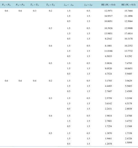
4.2. Relative Efficiency When Rare Unrelated Attribute Is Unknown
Let V2
( )
λˆA be the variance of the proposed estimator λˆA for the rare sensitive attribute when the parameter of rare unrelated attribute is unknown. The relative efficiency of proposed estimator with respect to( )
2 ˆ
A L
V λ
Figure 1. Relative Efficiency (RE) of the proposed model with respect to Lee et al. [4] for W1 = 0.4 and P12 = 0.3 to 0.8.
( )
( )
[
]
[
]
[
]
(
)
{
}
{
(
)
}
2
1 2
2
1 1 1
2
2 2
1 2
2
2 1
1 1 2 1 1 2
ˆ
ˆ
1 1
h h
h
A h h h
L
h h
A
h h
h h h h h h
A A
W
V P T
RE
A A
V
W
P P P T T T
λ λ
=
=
′ + ′
−
= =
+
+ − − + −
∑
The relative efficiency of proposed estimator is free from the sample size n. For the analysis, the design probabilities are fixed as P11=P21, P12=P22, T11=T21, T12=T22. Setting λ1A=λ2A, λ1Y =λ2Ywith parameter
values of
(
λ λ1A, 1Y)
,(
λ λ2A, 2Y)
as(
0.5,1.5 , 1.5, 0.5 , 1.5,1.5) (
) (
)
and P11=0.6, T11=0.3, 0.4, T12 = 0.2, 0.3,0.4, 0.5 and W1=0.4, 0.5
(
W1+W2=1)
. The relative efficiencies are given in Table 2 depict that the proposed estimator outer perform than( )
2 ˆ
A L
V λ estimator having efficiency greater than 1 if we set the probabilities as
12 12
P ≥T . However the relative efficiency starts decreasing as we take P12<T12. A study of Figure 2 confirms
[image:9.595.90.537.196.700.2]this. Also, when W1 increasesthe relative efficiency of proposed estimator increases.
Table 1. Relative efficiency of the proposed estimator with Lee et al. (2013).
W1 = 0.4 W1 = 0.6
P12 λ1Y λ1A P11 = 0.6 0.7 0.8 0.9 P11 = 0.6 0.7 0.8 0.9
0.3 0.5 1.5 1.7346 1.5829 1.4758 1.3966 1.5630 1.4264 1.3299 1.2585
1.5 1.5 1.9238 1.7016 1.5439 1.4266 1.7336 1.5334 1.3912 1.2855
1.5 0.5 2.2198 1.9173 1.6887 1.5016 2.0003 1.7277 1.5217 1.3531
0.4 0.5 1.5 1.8713 1.6667 1.5228 1.4169 1.6863 1.5018 1.3723 1.2768
1.5 1.5 2.1435 1.8333 1.6166 1.4574 1.9316 1.6520 1.4567 1.3133
1.5 0.5 2.6070 2.1568 1.8251 1.5615 2.3492 1.9436 1.6447 1.4071
0.5 0.5 1.5 2.0097 1.7510 1.5701 1.4372 1.8109 1.5779 1.4148 1.2951
1.5 1.5 2.3751 1.9699 1.6908 1.4885 2.2100 402 1.7751 1.5327 1.3413
1.5 0.5 3.0537 2.4245 1.9727 1.6238 2.7517 2.1848 1.7776 1.4633
0.6 0.5 1.5 1.6090 1.01489 1.2107 1.0910 1.9370 1.6545 1.4576 1.3135
1.5 1.5 1.9600 1.4204 1.3225 1.1377 2.3596 1.9026 1.5921 1.3698
1.5 0.5 2.6727 1.6326 1.5961 1.2642 3.2177 2.4550 1.9215 1.5219
0.7 0.5 1.5 1.7147 1.4383 1.2464 1.1063 2.0642 1.7315 1.5005 1.3318
1.5 1.5 2.1511 1.6900 1.3806 1.1616 2.5897 2.0346 1.6621 1.3984
[image:9.595.88.540.211.692.2]1.5 0.5 3.1223 2.2915 1.7258 1.3150 3.7592 2.7587 2.0776 1.5831
Figure 2. Relative Efficiency (RE) of the proposed model with respect to Lee
Table 2. Relative efficiency of the proposed estimator with Lee et al. (2013), W1 = 0.4, and W1 = 0.5.
P11 = P21 P12 = P22 T11 = T21 T12 = T22 λ1A = λ2A λ1Y = λ2Y RE (W1 = 0.4) RE (W1 = 0.5)
0.6 0.6 0.3 0.2 1.5 0.5 12.5971 15.7464
1.5 1.5 16.9517 21.1896
0.5 1.5 10.0051 12.5064
0.3 1.5 0.5 10.3926 12.9908
1.5 1.5 13.9851 17.4814
0.5 1.5 8.2542 10.3178
0.4 1.5 0.5 8.1881 10.2352
1.5 1.5 11.0186 13.7732
0.5 1.5 6.5033 8.1292
0.5 1.5 0.5 5.9836 7.4795
1.5 1.5 8.0520 10.0651
0.5 1.5 4.7524 5.9405
0.6 0.6 0.4 0.2 1.5 0.5 3.1703 3.9629
1.5 1.5 4.4483 5.5603
0.5 1.5 2.7607 2.4509
0.3 1.5 0.5 2.5759 3.2198
1.5 1.5 3.6142 4.5178
0.5 1.5 2.2431 2.8038
0.4 1.5 0.5 1.9814 2.4768
1.5 1.5 2.7801 3.4752
0.5 1.5 1.7254 2.1568
0.5 1.5 0.5 1.3870 1.7338
1.5 1.5 1.9461 2.4326
0.5 1.5 1.2078 1.5098
5. Conclusion
In this study, a two stage randomized response model is proposed with improved estimators for the mean and its variance of the number of persons possessing a rare sensitive attribute based on stratified sampling by using Poisson distribution. It is shown that our proposed method have better efficiencies than the existing randomized response model, when the parameter of rare unrelated attribute is known and in unknown case, depending on the probability of selecting a question. For future work, we can obtain more sensitive information from respondents by using stratified double sampling with the proposed model.
References
Computational and Graphical Statistics, 60, 63-66. http://dx.doi.org/10.1080/01621459.1965.10480775
[2] Greenberg, B.G., Abul-Ela, A.L.A., Simmons, W.R. and Horvitz, D.G. (1969)The Unrelated Question Randomized Response Model: Theoretical Framework. Journal of the American Statistical Association, 64, 520-539.
http://dx.doi.org/10.1080/01621459.1969.10500991
[3] Mangat, N.S. and Singh, R. (1990) On the Confidentiality Guaranteed under Randomized Response Sampling: A Comparison with Several New Techniques. Biometrical Journal, 40, 237-242.
[4] Lee, G.S., Uhm, D. and Kim, J.M. (2013) Estimation of a Rare Sensitive Attribute in a Stratified Sample Using Poisson Distribution. Statistics, 47, 685-709. http://dx.doi.org/10.1080/02331888.2011.625503
[5] Chaudhuri, A. and Mukerjee, R. (1988) Randomized Response: Theory and Techniques. Marcel Dekker, New York.
[6] Mahmood, M., Singh, S. and Horn, S. (1998) On the Confidentiality Guaranteed under Randomized Response Sam-pling: A Comparison with Several New Techniques. Biometrical Journal, 40, 237-242.
http://dx.doi.org/10.1002/(SICI)1521-4036(199806)40:2<237::AID-BIMJ237>3.0.CO;2-N
[7] Land, M., Singh, S. and Sedory, S.A. (2012) Estimation of a Rare Sensitive Attribute Using Poisson Distribution.
Sta-tistics, 46, 351-360. http://dx.doi.org/10.1080/02331888.2010.524300
![Figure 1. Relative Efficiency (RE) of the proposed model with respect to Lee et al. [4] for W1 = 0.4 and P12 = 0.3 to 0.8](https://thumb-us.123doks.com/thumbv2/123dok_us/8000681.761523/8.595.96.530.80.623/figure-relative-efficiency-proposed-model-respect-lee-et.webp)