Technological advances in imaging riometry

(1)

Lancaster University United Kingdom

Technological Advances in Imaging Riometry

Martin Grill, Dipl.-Ing. (FH)

Submitted in part fulfilment of the requirements for the degree of Doctor of Philosophy

(2)

Abstract

Technological Advances in Imaging Riometry

Martin Grill, Dipl.-Ing. (FH)

Submitted for the degree of Doctor of Philosophy June 2007

Since their inception in 1935, relative ionospheric opacity meters (riometers) have evolved through several generations, from simple, manually operated, widebeam receivers to automated multi-beam imaging riometers. This thesis follows the development of a new type of imaging riometer based on a Mills Cross antenna array: the Advanced Rio-Imaging Experiment in Scan-dinavia (ARIES). This is the first time that a digital cross-correlation beamforming technique has been used in riometry. The investigations presented cover initial simulations, software spec-ification, design and implementation, hardware prototyping, the working instrument and first data products. Therefore, the work is an interdisciplinary slice through the engineering cycle of ARIES, encompassing a variety of subject areas, including (Space Plasma) Physics, Electronics, Astronomy and (Software) Engineering.

This thesis makes three specific contributions. Firstly, several low- and high-level simula-tions are presented, culminating in the development of the riometer simulation toolkit (RIOSIM). RIOSIM is not specific to ARIES, but is capable of simulating the behaviour of arbitrary antenna arrays.

Secondly, a flexible software architecture is developed and implemented in form of the Ad-vanced Riometer Components (ARCOM) operating software. ARCOM consists of components

(3)

streaming data format based around principles similar to those used in digital video broadcast-ing (DVB). ARCOM software architecture and data formats are not limited to riometry but will readily support a wide range of data acquisition and processing tasks.

(4)

Declaration

The material presented in this thesis is the result of my own work and has not been produced as the result of collaborations, except where specifically indicated. The material has not been submitted in substantially the same form for the award of a higher degree elsewhere.

Some of the ideas in this thesis stem from discussions with my supervisors and colleagues, and these have been referenced as ‘personal communication’ where appropriate.

Some of the material presented in this thesis has been, or is in the process of being, published in journals (Hagfors, Grill, Honary 2003 — [HGH03]; Nielsen, Honary, Grill 2004 — [NHG04]; Honary, Grill, Barratt, Nielsen 2007 — [HGBC07]) and conference presentations (Grill, Honary, Nielsen et al. 2003 — [GHN+03]; Honary, Marple, Kosch, Senior, Makarevitch, Grill 2004 — [HMK+04]; Barratt, Honary, Grill, Chapman 2004 — [BHGC04]; Grill, Senior, Honary 2005 — [GSH05]; Honary, Chapman, Grill, Barratt et al. 2005 — [HCG+05]; Honary, Chapman, Grill, Barratt et al. 2006 — [HCG+06]).

Martin Grill

(5)

“To him who is able to do immeasurably more than all we ask or imagine, according to his power that is at work within us.” [God]

(6)

Acknowledgements

While working on this thesis, numerous people have supported and influenced me in many different ways. Mentioning them all seems even more of a ‘Wicked Problem’ than designing operating software for ARIES. So I shall ask forgiveness from all those people I have missed out on the following list and from those whose contributions I have misrepresented or misjudged.

Stefani Maier and Haybatolah Khakzar have helped establish the contact with Lancaster University in the first place. I thank my supervisor Farideh Honary for giving me the opportunity to write this thesis and supporting me all the way.

Erling Nielsen and the late Tor Hagfors are the originators of the idea to build a riometer based around a Mills Cross antenna array.

Hisao Yamagishi suggested a valuable practical approach for integration time estimation. Mike Rietveld and staff at the EISCAT facility near Tromsø have helped out with advice and equipment on various occasions, both during our on-site campaigns in Norway and during remote operation.

As well as being a brilliant role model of a scientist and the originator of the ideas behind chapter 10, Andrew Senior has often supported me with advice, comments and uniquely insight-ful, ethical and diplomatic points of view. He has also provided me with much-needed extra time by taking over some of my duties at various times.

Throughout several projects, including ARIES, Keith Barratt has always been a pleasure to work with and an invaluable source of advice. He also shared my passion for well-designed systems and interfaces.

Peter Chapman was the source of many interesting insights into RF design and applied elec-tronics.

The support and friendship of all members of the Space Plasma Environment and Radio Sci-ence (SPEARS) group has always been a great encouragement and especially Roman Makare-vitch has become a good friend.

(7)

Council (PPARC), which has since been merged into the Science and Technology Facilities Council (STFC). Without funding for the ARIES project, this thesis would not have been possi-ble.

I am deeply grateful that my parents Wolfgang and Sibylle Grill and my sister Claudia Grill have been a never ending source of love and support.

Martin and Claudia Strohbach have become dear friends and have provided valuable advice, support and my first godchild!

My church family at Lancaster Baptist Church and beyond, and particularly our housegroup, have been a tremendous source of strength, support and advice.

(8)

List of Figures

2.1 A simple phased array . . . 10

2.2 Beamforming summation . . . 10

2.3 Beams formed by a 32 port Butler Matrix . . . 13

2.4 Two different ways of cosine tapering for a 32 element linear array . . . 13

2.5 Beam pattern for cosine tapered input signals . . . 14

2.6 Beam pattern for ‘half’ cosine tapered input signals . . . 14

2.7 Pairwise addition of Butler Matrix outputs . . . 15

2.8 Beam pattern of a 32 port Butler Matrix with outputs added pairwise . . . 15

2.9 Original Mills Cross . . . 19

2.10 Beamforming for a Mills Cross . . . 19

2.11 Signal-processing view of reception of signals by a Mills Cross . . . 24

3.1 Trace of IRIS beam 31 during one sidereal day . . . 27

3.2 IRIS QDC and recorded power for 2002-10-30 . . . 29

3.3 IRIS absorption for 2002-10-30 . . . 29

3.4 Complexity of widebeam, phased array and Mills Cross type riometers . . . . 31

3.5 Physical layout of several Mills Cross and filled array antenna configurations 33 3.6 Long-distance view of ARIES . . . 33

3.7 Close-up view of ARIES . . . 34

3.8 Inside the ARIES control hut . . . 34

3.9 The atmosphere of the Earth . . . 43

3.10 Bright Radio Sources . . . 44

3.11 The part of the sky that affects ARIES/IRIS . . . 45

3.12 Sky temperature in K as mapped by Cane’s sky map . . . 47

3.13 Sky temperature in K as mapped by the GEETEE sky map . . . 47

(19)

4.2 ARIES system model, stage 1: Reception . . . 52

4.3 ARIES system model, stage 2: Beamforming . . . 52

4.4 ARIES system model, stage 3: Cross-correlation and integration . . . 55

4.5 Class diagram for ARIES model . . . 55

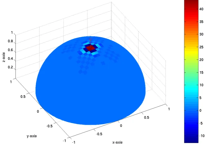
4.6 3 sources, 4×105samples . . . 59

4.7 10 sources, 4×105samples . . . 59

4.8 The same 20 sources, different integration times . . . 60

4.9 Phase centre issues . . . 63

4.10 Effect of pure sinusoidal sources . . . 64

4.11 ‘Negative sidelobes’ . . . 67

5.1 Class diagram for noise sources in Yamagishi Model . . . 71

5.2 Two intersecting fan beams . . . 74

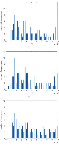
5.3 Measurement example . . . 74

5.4 Normalised simulation results . . . 76

5.5 Simulation results for different quantities of simulated noise sources . . . 78

5.6 Influence of incoherently received power on the integration time. Part 1 . . . 80

5.7 Influence of incoherently received power on the integration time. Part 2 . . . 80

5.8 Effect of different boundary conditionsεon integration time . . . 83

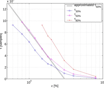
5.9 Required integration time to measureτ30%,τ50%,...,τn% . . . 85

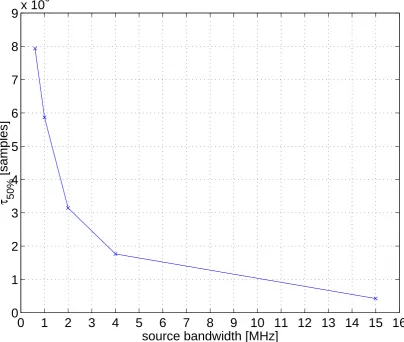
5.10 Required integration time in samples versus system bandwidth . . . 86

5.11 Required integration time in samples versus sampling rate . . . 88

6.1 RIOSIM architecture . . . 97

6.2 RRadPat and descendants . . . 97

6.3 Basic plotting capabilities of a RRadPat radiation pattern object . . . 100

6.4 Advanced 3D visualisation options . . . 103

6.5 Some RRadPat-derived radiation patterns. . . 103

6.6 Radiation pattern of a crossed dipole above ground . . . 108

6.7 CSkyMap and descendants . . . 108

6.8 CTaohSkyMap vs. CGrillTaohSkyMap . . . 110

(20)

LIST OF FIGURES xx

6.10 ‘Projection 1’: Projection onto the ionosphere . . . 113

6.11 FLATM projection as used for IRIS image data . . . 118

7.1 ARIES and IRIS beam contours . . . 122

7.2 Multiple contour levels and radio star traces for 2001-01-20 . . . 124

7.3 IRIS power data for beam 38 on 2001-01-20 . . . 125

7.4 Theoretical QDCs for IRIS compared to real QDCs . . . 130

7.5 Simulated QDCs for the 716 ‘existing’ ARIES pencil beams . . . 132

7.6 One frame of the ARIES worst-case beam determination movie . . . 135

7.7 RP, the radiation pattern explorer . . . 135

7.8 Output of scint_calc_mia() for 20 January 2001 . . . 139

7.9 Three screenshots of the scintillation calculator . . . 143

7.10 Remote execution the hard way. Client side . . . 143

7.11 Remote execution the hard way. Server side . . . 147

8.1 Multi-layer view of ARCOM and its operating environment . . . 152

8.2 From spaghetti-code to distributed applications . . . 152

8.3 Structure of a CORBA-based application . . . 153

8.4 An example of pipelining: Pipes on the UNIX command line . . . 153

8.5 The three basic ARCOM (meta-)components . . . 156

8.6 ARCOM example configuration as used during initial experiments . . . 156

8.7 ARCOM example configuration for current FPGA-based design . . . 158

8.8 Example of ARCOM data flow through a shared memory interface . . . 158

8.9 AShMemInterface class hierarchy . . . 162

8.10 AShMemInterface states . . . 162

8.11 An ARCOM shared memory interface in use . . . 164

8.12 ALogFile and descendants . . . 173

8.13 ARCOMPACKET_FPGAPACKET . . . 175

8.14 ARCOM CORBA interfaces . . . 176

8.15 Life cycle of an ARCOM component . . . 176

8.16 gui1.tcl: A simple GUI for controlling ARCOM components . . . 187

9.1 Hardware available during the October 2002 experiment . . . 196

(21)

9.4 Difference between post-integrating (complex) raw data and post-integrating

preprocessed data . . . 205

9.5 Beam width versus integration time (zenithal beam) . . . 206

9.6 Receiver working range and signal dynamic range . . . 208

9.7 Influence of the strong radio stars . . . 214

9.8 The radio stars’ influence on beam 3501. Part A: fan beams . . . 215

9.9 The radio stars’ influence on beam 3501. Part B: pencil beam . . . 216

9.10 Amplitude and phase response of a 16-element linear phased array . . . 216

9.11 Pencil beam comparison for multiple days . . . 217

9.12 ARIES / IRIS beam projections onto different heights . . . 218

10.1 Non-interpolated IRIS and ARIES data for 2007-03-20 08:45 . . . 223

10.2 ‘Traditional’ IRIS image interpolation . . . 223

10.3 Obliquity factorδcorrecting for apparent thickness of absorption layer . . . . 228

10.4 Inter-relations of the parametrised interpolation model method (GLEAM) . . 228

10.5 Examples of direct orthogonal basis functor fits . . . 230

10.6 The first 49 real spherical harmonics . . . 233

10.7 Influence of compression factor on ‘adjusted’ spherical harmonic fit . . . 233

10.8 GLEAM class diagram . . . 235

10.9 GLEAM with simulated ARIES data; Constellation 1 . . . 237

10.13 Visualisation of the traditional image interpolation algorithm for ARIES . . . 244

10.14 Performance of the traditional interpolation method for three cases . . . 245

10.15 Path of a simulated absorption patch across a ‘frozen’ sky map . . . 246

10.16 Simulated power readings during absorption event . . . 246

10.17 Diurnal variation of model weighting coefficients for direct sky map fit . . . . 253

10.18 ARIES real and simulated complex beam data for 12 exemplary beams . . . . 254

10.19 Sequence of ARIES power images for 2007-03-23 . . . 255

(22)

LIST OF FIGURES xxii

10.21 Sequence of ARIES power images for absorption event . . . 257

11.1 Advanced ARCOM deployment examples supporting real-time data feeds . . 267

B.1 Common coordinate systems . . . 281 B.2 Conversion from geographic to horizontal coordinates . . . 289

D.1 ARIES block diagram . . . 296 D.2 ARIES receiver block diagram . . . 297 D.3 ARIES receiver PCB . . . 297 D.4 ARIES FPGA data flow . . . 298 D.5 ARIES physical layout . . . 299

G.1 ARIES ‘earlobe’ plots: all central 676 beams . . . 308 G.2 Zoomed-in version of figure G.1, part 1 . . . 309 G.3 Zoomed-in version of figure G.1, part 2 . . . 310 G.4 Zoomed-in version of figure G.1, part 3 . . . 311 G.5 Zoomed-in version of figure G.1, part 4 . . . 312 G.6 Zoomed-in version of figure G.1, part 5 . . . 313 G.7 Zoomed-in version of figure G.1, part 6 . . . 314

(23)

3.1 Summary of discussed sky maps . . . 43

4.1 Available command line arguments formodel . . . 55

5.1 Noise sources used in ARIES simulations . . . 71 5.2 Simulations to determine the influence of the number of noise sources . . . 80 5.3 Simulations with sources of different intensities . . . 82 5.4 Simulations with different boundary conditionsε . . . 82 5.5 Simulations with different bandwidths . . . 85 5.6 Simulations with different sampling rates . . . 88 5.7 Summary of integration time estimates . . . 92

8.1 Comparison of three common componentry frameworks . . . 153 8.2 ARCOM packet types . . . 173 8.3 ARCOM descriptor types . . . 174 8.4 ARCOM component status values . . . 174 8.5 ARCOM low-level shared memory tools . . . 187 8.6 Important ARCOM component files . . . 191 8.7 ARCOM files in theARCOM/common/directory . . . 193

9.1 Available datasets as recorded during October 2002 experiment . . . 196 9.2 Achievable accuracy for different integration times . . . 205

10.1 Summary of GLEAM performance with simulated ARIES data . . . 242

B.1 Common coordinate systems . . . 277

C.1 Timescales (1) . . . 293

(24)

LIST OF TABLES xxiv

(25)

Introduction

New technologies enable us to probe as-yet unknown areas of creation. Today’s complex sys-tems are made up of a multiplicity of mechanical, electrical and electronic components, with the intangible ‘ether’ of software causing dead matter to rise beyond its pure existence and assist us in our quest of exploration. It is this fascination with making things work, interact and fulfil a higher purpose that drives an engineer.

This thesis follows the development of a new type of imaging riometer based around the principle of a Mills Cross cross-correlating antenna array: the Advanced Rio-Imaging Experi-ment in Scandinavia (ARIES). This is the first time that a digital cross-correlation beamforming technique has been used in riometry.

The author’s background in Mechatronics results in this thesis being an interdisciplinary slice through the engineering cycle of ARIES, encompassing a variety of subject areas including (Space Plasma) Physics, Electronics, Astronomy and (Software) Engineering.

Several of the concepts presented in this thesis have since been applied to, or used during the development of, other scientific instruments. These include the Advanced Imaging Riometer for Ionospheric Studies (AIRIS), which uses the ARCOM operating software, and the new high-speed photometer for optical emission measurements (SPARKLE), which employs a packet-based streaming data format very similar to the one presented in this thesis.

1.1 Main Contributions

This thesis makes three specific contributions. Firstly, several low- and high-level simulations are presented, culminating in the development of the riometer simulation toolkit (RIOSIM).

(26)

CHAPTER 1. INTRODUCTION 2

RIOSIM is not specific to ARIES, but is capable of simulating the behaviour of arbitrary antenna arrays.

Secondly, a flexible software architecture is developed and implemented in form of the Ad-vanced Riometer Components (ARCOM) operating software. ARCOM consists of components participating in processing pipelines through high-speed shared memory interfaces and a flexible streaming data format based around principles similar to those used in digital video broadcast-ing (DVB). ARCOM software architecture and data formats are not limited to riometry but will readily support a wide range of data acquisition and processing tasks.

Thirdly, a new approach to image interpolation for riometers (GLEAM) is developed and its performance evaluated. GLEAM uses a matrix inversion technique, combined with knowledge about antenna and phased array directivity patterns and predictions obtained from simulations, to fit a parametrised model of the sky brightness distribution to real data. This is envisaged to become the primary data product of a new generation of riometers.

1.2 Brief Description of All Chapters

The sequence of chapters follows the logical development cycle of the riometer, from inital con-cepts through low- and high-level simulations, software specification, design and implementa-tion, hardware prototyping and testing to a sophisticated piece of scientific measuring equipment and analyses of real data recorded by this brand-new instrument. Each chapter builds on the pre-ceding ones. Chapters 2 and 3 form the background part of the thesis, the subsequent chapters address the author’s specific contributions. Additional information to complement the material presented in the main body of the thesis is provided in several appendices, including technical documentation of certain tools as well as information collated from third-party documentation that is not the author’s own work, or only distantly related to the main topic of this thesis.

Antennas are essential in any device that receives or transmits radio waves.Chapter 2looks at properties of individual antennas as well as of arrays of antennas. This general description forms the basis for the more specific discussion of our area of interest, riometry, and how anten-nas are used in riometers, in chapter 3. A large part of chapter 2 is dedicated to the discussion of various aspects of the Mills Cross as used by the Advanced Rio-Imaging Experiment in Scandi-navia (ARIES) riometer.

(27)

de-chapter 2. Sky maps and radio stars are also introduced and basic concepts relating to these are discussed. Knowledge about the working principles of riometers, sky maps and radio stars is important for the chapters to follow.

Inchapter 4we introduce a set of programs to simulate the data flow through a Mills Cross type system from source to the final beam output. These programs (and the results they produce) help to deepen the understanding of the working principle of a Mills Cross type system such as the one used for ARIES. The simulations discussed in this chapter will also enable us to examine the signals inside the system at various stages, providing test data even before any hardware has been built.

The fact that this simulation is done at signal level implies that it is not possible to simulate long periods of time due to the amount of processing power and storage space required. For the same reasons, the simulation cannot be carried out in real-time, and there is a practical limit to the number of sources that can be simulated.

Chapter 5will introduce a different simulation that is geared towards determining estimates for the required integration time in a realistic situation, but these simulations will no longer simulate the whole reception process (as done in chapter 4) but only the final cross-correlation stage. We explore how different factors contribute to the required integration time, these results are then used to extrapolate a realistic estimate of the required integration time.

Having looked at the basic working principles of antennas and riometers in chapters 2 and 3, and having simulated the low-level reception processes in chapters 4 and 5,chapter 6 oper-ates on a higher level of abstraction, focusing on radiation patterns and on how the concept of radiation patterns can help in the evaluation and deployment of real system designs.

The toolbox developed in this chapter will enable us to apply all findings to arbitrary riome-ters or, in fact, antenna systems.

(28)

CHAPTER 1. INTRODUCTION 4

toolkit, the power of many of the applications presented can easily be harnessed for other riome-ters, usually by simply changing the location, time and beam pattern parameters appropriately.

Chapter 8defines the ARCOM framework, a generic operating software for advanced ri-ometer systems. The chapter is roughly structured along the process activities of the Software Engineering cycle. It does not go into implementation details of every single function call, aim-ing instead at providaim-ing a general (although more abstract) description of the workaim-ing principles involved.

The design of operating software for a ‘Wicked System’ such as ARIES presents unique challenges to the software engineer. The chapter looks at what these challenges are, how they influenced the design of the ARIES operating software, and how the implemented software architecture solves the ‘Wicked Problem.’

Chapter 9contains discussions of the different results obtained from the 2002 ARIES ex-periment. During the 2002 experiment, a variety of datasets has been recorded for different configurations of a preliminary ARIES system. The data comprises several hundred gigabytes of raw input data as recorded from the A/D converters connected to the beamforming network, as well as integrated data derived from the raw data in real-time.

The first full ARIES system started recording first long-term datasets in March 2006, and data from ARIES in its final configuration is available from March 2007.Chapter 10describes the GLEAM algorithm developed to compensate for the correlation-related issues discovered during the initial experiments. This algorithm also has the potential to provide higher-quality image interpolation compared to the currently used approach. We describe the GLEAM algo-rithm and apply it to various test- and real datasets to show its effectiveness.

Chapter 11summarises the thesis, and draws some conclusions for future development of riometers. The results presented in this thesis open up many new research opportunities, and some ideas for future work are presented.

(29)

The layout of this thesis adheres to the official guidelines of the University of Lancaster as published in [Par07]. In the electronic (PDF) version of this document, all (cross-)references have been hyperlinked for reading convenience. The following typographical conventions are used throughout this thesis:

• Variable parameters in equations are depicted by lowercase italic characters, e.g.n.

• BoldC-style notation is used for program functions (methods), i.e. run().

• Classes, objects, components and variables are referred to inbold text, but without trailing parentheses, as inCNoiseSource.

• Boldanditalictext is also used for general emphasis.

• Where deduction from the context is potentially ambiguous, the C++-style scope operator (::) is used to indicate which class a function belongs to, for example CNoiseSource::-getSample().

• Amonospaced fontis employed for

– File names (e.g.small_circle.source).

– File contents.

– Output of commands.

– (Excerpts of) source code.

• Abold monospacedfont is used for commands and names of programs entered on a command line (e.g../sendcmd).

(30)

Chapter 2

Antennas

Antennas are essential in any device that receives or transmits radio waves. This chapter sum-marises some properties of individual antennas as well as of arrays of antennas in general. This general description forms the basis for the more specific discussion of our area of interest, riom-etry, and how antennas are used in riometers in chapters 3 onwards.

2.1 Radiation Properties of Antennas

Antennas radiate or receive energy in form of electromagnetic waves. The radiation pattern of an antenna describes how the antenna in question responds to radiation received from any given direction. The radiation pattern of an antenna usually depends on the frequency of the radiation in question. Antennas can be designed to maintain a nearly constant radiation pattern over a wide range of frequencies. However, most simple antennas show strong variations in their radiation pattern as the operating frequency is varied.

From the description above it is clear that at least two parameters are needed to describe the radiation pattern of any given antenna, namely the spherical coordinates (azimuth and elevation) that specify the direction in question.

However, electromagnetic radiation can be polarised. To fully describe a radio wave propa-gating in any given direction, the polarisation state of this wave needs to be known. This can be specified through the Stokes parameters [Kra88], or, equivalently, through two complex phasors in space quadrature describing the two principal components of the electric field (or equivalently the magnetic field which is always perpendicular to the electric field) and the relative phase offset between them.

(31)

on, we will refer to such a radiation pattern as complex radiation pattern, because two (complex) phasors are used to describe the radiation properties for each direction.

Most of the time, however, one is not interested in the instantaneous amplitude of the re-ceived signal. The property of interest is the average power rere-ceived from any given direc-tion. This is called the power gain of an antenna (often specified in relative terms relative to an ‘isotropic radiator’ and assuming unpolarised radiation). Another term that is often used to describe the properties of an antenna is the ‘antenna directivity.’ Often, this refers to the power gain as discussed above. Sometimes, the term directivity is also used to describe themaximum power gain.

2.2 A Brief History of Crossed Dipole Antennas

The individual antenna elements of today’s riometers are crossed dipole antennas, also known as ‘turnstile’ antennas. This kind of antenna was first described by Brown in [Bro36]. Brown’s goals were to build an antenna with circularly symmetrical radiation pattern that should concen-trate the energy in the vertical plane so that the signal strength toward the horizon for a given power input will be considerably greater than that obtained from a single half-wave vertical an-tenna with the same input power. In fact, he built a vertical array of what we now know as crossed dipole antennas. In [Bro36], he also derives the horizontal radiation pattern of such an antenna, and how it changes as a function of the amplitude and phase of the signal that is fed into each of the two arms of the crossed dipole. He experimentally verified the uniformness of the radiation pattern if the current in the two arms is in time quadrature.

(32)

CHAPTER 2. ANTENNAS 8

today’s MIMO (multiple input multiple output systems) which are used in digital communication systems [SCT03].

Wells [Wel44] describes a ‘quadrant aerial’ consisting of two linear dipoles in space quadra-ture. He describes the radiation patterns of such an antenna for different lengths of dipoles. He also derives radiation patterns for such antennas above perfect and imperfect earth. The two dipoles of his ‘quadrant aerial’ are, however, not centred on each other. Their common point is located at the end of the dipoles.

Today, crossed dipoles are widely used in riometry. The main reasons are

• Omnidirectional radiation pattern.

• Circular polarisation matches predominant polarisation of incoming ‘signal’ from cosmic noise background.

• Simple and inexpensive to build [Nie01].

• Use of guy ropes (IRIS) or guide wires (ARIES) makes them highly resistant to environ-mental influences such as snow and wind.

In [Nie01], Nielsen approximates the power gainψof such a crossed dipole to be

ψ=2·sin(2π λ h·sin(

π

2−θ)) (2.1)

where λ is the wave-length, h the height of the antenna in wave-lengths above a perfect ground plane andθthe zenith angle. We can visualise this and other radiation patterns with the RIOSIM toolkit described in chapter 6.

2.3 Phased Array Antennas

2.3.1 Working Principle of an Additive Phased Array

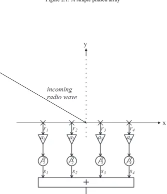
Figure 2.1 shows a simple example of an additive phased array. The antenna elements are posi-tioned in a Cartesian coordinate system, the location of each elementiis described by its position vector−→pi. All lengths are specified in multiples of the operating wavelength. In figure 2.1, for

(33)

To understand the response of such an array to an arbitrary incoming radio wave, we logically divide the process up into the reception (this section) and beamforming (section 2.3.3 below) stages.

Let the direction of the incoming wave be specified by the unit vector−→w. If we want to find the directivity pattern of the array, we simply have to determine the response of the array to all possible incoming wave directions−→w. That is why, in the following discussion, we stick to one single direction−→w =−w→0.

A wave received from a certain direction−→w is received by each aerial with a certain phase shift relative to the centre of the array (or, in fact, any arbitrary fixed point in space — known as the phase centre1). This individual phase shift depends on the placement−→pi of the aerial element

iin question and on the direction of the incoming wave as specified by−→w.

Note that all phase information is relative to a certain fixed point and time, for convenience we specify that point to be the origin of the coordinate system. Thus, an aerial atO(0|0|0)

receives the wave from direction−→w with phase delay 0rad=0◦. We will specify all angles in radians from now on.

The amount of phase delay for any given aerial position−→pi is simply related to the projection

of−→pi on the direction vector−→w of the incoming wave:

∆φi=−2π· −→w· −→pi (2.2)

This relation is also shown in figure 2.1, again for a simple two-dimensional case.

2.3.3 Additive Beamforming

In order to form a beamnpointing into a specific direction, the input signals are added together (thus additive array) with certain additional phase shiftsβi,n. These phase shifts determine the

direction of the formed beam. Figure 2.2 shows this process for one specific beam. In addition, the signal from each individual antenna element can be attenuated by a certain amount, again affecting the shape and direction of the resulting beam. This step is known as tapering, and a variety of tapering functionsa(−→pi) exist, leading to different sidelobe levels and beam widths.

Theoretically, one could specify an individual tapering function for each beam. In practice, one 1_{To obtain correct results when adding the response from several (sub-)arrays, it is important that their phase}

(34)

x

y

w

p

₁

D f

d i r e c t i o n o f i n c o m i n g

r a d i o w a v e

1

[image:34.595.150.485.310.700.2]

2 p

Figure 2.1: A simple phased array

x

y

i n c o m i n g

s

3

s

4

(35)

Mathematically, this reception and beamforming process can be described as follows: Reception of signal by all aerialsi:

ri=e−j·2π·−

→

w·−→pi _(2.3)

Attenuate signal and apply phasing:

si=ri·ai·e−j·βi,n (2.4)

Add up all components to form the beam:

S=

_∑

si (2.5)

2.3.4 Phase Angles for Butler Matrices

Butler Matrices use an optimised network of phase shifters to form multiple simultaneous beams from a phased array antenna [BL61, Mue72]. Systematic methods are available to design Butler Matrices of any size 2N _{[Moo64]. A ‘standard Butler Matrix’ with} _N

in inputs has an equal

number of outputsNout=Nin=N, thus produces Nbeams. A Butler Matrix is normally used

with linear arrays with equally spaced elements connected to its inputs{1, . . . ,N} and applies the following phase factors:

βi,n=

i−N+1 2

·(n−1)−

N−1 2

N

2

·π (2.6)

where the term (n−1)−

N−1 2 N 2

·πis the phase progression from element to element for a given beam number, and i−N+1

2

(36)

2.3.5 Cosine Tapering

Tapering (i.e. attenuating) the signals from the individual antenna elements leads to differently shaped beams. In general, the aim of tapering is to reduce the sidelobes. The drawback is that the main beam is broadened in doing so.

If, for example, we taper the individual signals according to a cosine function as shown in figure 2.4, the resulting beam pattern for the same Butler Matrix as in 2.3.4 will look like in figure 2.5. Again, beam 9 is highlighted, and it is clearly wider than the original beam 9 in figure 2.3. At the same time, however, the level of the first sidelobes is reduced to−32dB.

Other forms of cosine tapering are possible, for example according to the dotted line in figure 2.4. This will lead to the beam pattern shown in figure 2.6.

The formula that was used to calculate the attenuation factors for the continuous line in figure 2.4 is

ai=

1 2 cos

i−N+1 2

N−1 2 ·π

!

+1

!

(2.7)

Formula 2.8 below was used for the dotted line in figure 2.4.

ai=

1 4 cos

i−N+1 2

N−1 2 ·π

!

+3

!

(2.8)

2.3.6 Pairwise Addition

As Nielsen suggests in [Nie02b], with reference to [Mue72], a beam pattern similar to the one in figure 2.6 can be achieved by pairwise addition of the output ports of a 32 port Butler Matrix using 16 signal combiners connected to the 32 output ports of the Butler Matrix, as shown in figure 2.7. This leaves us with 16 beams, the beam pattern of which looks like in figure 2.8. Clearly, there is some resemblance between figures 2.8 and 2.5. Pairwise addition of output ports therefore leads to similar results to cosine-shaped tapering, but without the need of additional attenuators in the input signal lines, therefore reducing overall signal loss.

(37)

0 10 20 30 40 50 60 70 80 90 100 110 120 130 140 150 160 170 180 −40 −35 −30 −25 −20 −15 −10 −5 0 1

elevation angle [°]

power [dB]

2 3 4 5 6 7 8 1011121314151617181920212223242526272829 30 319 32

Figure 2.3: Beams formed by a 32 port Butler Matrix connected to a linear antenna array. Cut along the vertical plane containing the antenna elements.

1 3 5 7 9 11 13 15 17 19 21 23 25 27 29 3132

0 0.1 0.2 0.3 0.4 0.5 0.6 0.7 0.8 0.9 1 antenna element attenuation factor Cosine Tapering

(38)

CHAPTER 2. ANTENNAS 14 0 10 20 30 40 50 60 70 80 90 100 110 120 130 140 150 160 170 180 −40 −35 −30 −25 −20 −15 −10 −5 0 1

power [dB]

Beampattern

2 3 4 5 6 7 8 1011121314151617181920212223242526272829 30 319 32

Figure 2.5: Beam pattern for cosine tapered input signals. Note that the level of the first sidelobes is reduced to−32dB.

0 10 20 30 40 50 60 70 80 90 100 110 120 130 140 150 160 170 180 −40 −35 −30 −25 −20 −15 −10 −5 0 1

power [dB]

Beampattern

2 3 4 5 6 7 8 1011121314151617181920212223242526272829 30 319 32

(39)

f r o m a e r i a l s

B u t l e r M a t r i x

+

b e a m s

+

Figure 2.7: Pairwise addition of Butler Matrix outputs

0 10 20 30 40 50 60 70 80 90 100 110 120 130 140 150 160 170 180 −40 −35 −30 −25 −20 −15 −10 −5 0 1

power [dB]

Beampattern

2 3 4 5 6 7 8 9 10 11 12 13 14 15 16

(40)

2.3.7 Conclusion

With additive phased arrays one can achieve highly directional antennas. These arrays tend to suffer from high sidelobe levels which can be reduced by tapering, in turn broadening the main lobe.

Pairwise addition of the Butler Matrix outputs seems to be an interesting alternative to atten-uating the input signals. It turns out, however, that the signal combiners needed to perform this pairwise addition are rather more expensive than attenuators.

Also, the pairwise addition method obviously leaves no flexibility for modifications, whereas the attenuator method enables one to shape the beams according to a multitude of tapering functions, cosine tapering (figure 2.4) being only one of many possibilities. Based on these results, it was decided to run initial ARIES Mills Cross experiments without using any kind of tapering. Though this will be of limited use for operation as a riometer later on, we can expect useful results from this configuration. In particular, we should be able to measure the high sidelobes of the untapered array, giving us confidence that the receiving system is working according to specification. The narrow, untapered pencil beams will also enable us to accurately measure the location of strong radio sources, and compare these measurements to theoretical simulations — thereby confirming correct alignment of the antenna array.

2.4 Mills Cross Antennas

2.4.1 A Brief History of Mills Cross Type Antenna Arrays

B. Y. Mills initially used three aerials connected together as Michelson-type interferometers [TMGWS86] at a frequency of 101MHz to examine the galactic distribution of discrete radio sources [Mil52]. Reasonable, albeit less than originally anticipated, accuracy was achieved, with an average probable error in position of around 0.2% for strong sources and 2% for weak sources.

What is now known as Mills Cross antenna is first described in [ML53]. Mills’s goal was to construct an aerial system of high resolution but small area and low cost for investigations in radio astronomy. Mills explicitly mentions that this kind of aerial system sacrifices gain (i.e. effective area) for high resolution and low cost. This was more than acceptable because Mills’s goal was to accurately map the positions of strong radio sources.

(41)

operating at 97MHz.

Having obtained encouraging results from this first system, Mills built a 250×2+250×2 element Mills Cross type radio telescope for use at 3.5m (86MHz) [MLSS58]. Other telescopes were developed at the same time, see for example [Sha58]. Christiansen and Mathewson used a Mills Cross antenna array to scan the solar disk at a wavelength of 21cm with unprecedented detail [CM58]. The interesting thing about this particular Mills Cross antenna is the fact that Christiansen did not care about sidelobes. He designed the array in such a way that the spacing between two adjacent lobes was large enough so that no two antenna lobes could fall on the sun at the same time. Note that Christiansen only used one pencil beam at any given time. He made successive scans of the sun during the course of several days to derive the brightness distribution across the whole solar disc. He also employed phase shifters in one of the two arms of his Mills Cross antenna array to steer the fan beam generated by this arm, therefore also changing the position of the resulting pencil beam.

2.4.2 Working Principle of a Mills Cross Antenna Array

The working principle of a Mills Cross antenna array is as follows.

2.4.2.1 Fan Beams

Initially, each arm of the cross is considered as a separate linear additive phased array (see section 2.3.1). Figure 2.9, panel (b) shows the idealised outline of the radiation patterns of the individual arms for the zenithal case. Each arm forms what is called a fan beam. The pointing direction of this fan beam can be influenced by appropriate phasing techniques such as the ones described in section 2.3.3. For example, if we have an arm of 32 antennas positioned half a wavelength apart from each other, and those antennas are connected to a 32 port Butler Matrix, we get 32 fan beams like the ones depicted in figure 2.3.

(42)

By themselves, the recordings from these fan beams are still rather useless. They cover a large solid angle, the spatial resolution (at least in one direction) is still very poor, in fact it equals the ‘resolution’ of a single antenna element. The direction of any signal recorded by such a fan beam can only be estimated in one direction, and only if no other interfering noise sources are present at the same time.

2.4.2.2 Cross-correlation, Pencil Beams

The idea that turns the Mills Cross antenna array into a high resolution array is based on cross-correlation of the signals from two perpendicular fan beams. This will extract only the signals that originate from the overlapping region of the two fan beams. A narrow pencil beam is therefore being formed for each combination of a fan beam from one arm with a fan beam from the other arm of the Mills Cross.

In case of a 32+32 antenna element Mills Cross array with a 32 port Butler Matrix for each arm, 32×32=1024 pencil beams are therefore being formed, though not all of them are physically meaningful, and even fewer perform well enough in terms of noise level and sidelobe behaviour to be suitable for further use. These issues will be discussed in more detail in subsequent chapters, primarily for one particular system, the Advanced Rio-Imaging Experiment in Scandinavia (ARIES).

Figure 2.10 is a 3D representation of the beamforming process. The two small panels on the left show an example of a fan beam formed by a linear array of antennas along the y-axis (top panel) and along the x-axis (bottom panel), respectively. The small inset in the upper right hand corner of each panel shows an idealised top-down view of several fan beams generated by the arm in question, with the shown fan beam highlighted.

(43)

Figure 2.9: Original Mills Cross, taken from [ML53]. (a) Plan view of dipoles in cross arrange-ment. (b) Idealised response of the cross arrangement, plan view.

(44)

2.4.3 Disadvantages of a Mills Cross

The following sections list well-known disadvantages of a Mills Cross antenna array when com-pared to a filled array. Note that these points don’t make a Mills Cross inferior to a filled array antenna, since superiority/inferiority always depends on the intended use of a system. Later on in this thesis we will investigate how these issues can be dealt with, and we will find that the Mills Cross still offers advantages over a filled array for use in riometry, mainly due to the by far smaller number of antenna elements required, translating into significant savings in terms of money and real estate.

2.4.3.1 High Sidelobe Levels

This section explains why the Mills Cross antenna array produces higher sidelobes than a cor-responding filled array for the untapered case. The Mills Cross forms the output signal of each pencil beam by cross-correlating the signals from two perpendicular fan beams generated by the two arms of the cross. The arms themselves are simple linear phased arrays and therefore produce a sidelobe level of around−13dB (in the untapered case).

Suppose, the received time series from the two perpendicular fan beams are called jt andkt,

respectively. Each signal has sidelobes, a source signal from the direction of the first sidelobe is therefore attenuated by−13dB in power. The signal itself, however, is therefore only attenuated by√−13dB.

The worst case happens when a source signalxtis received in the main lobe of one fan beam

and in the first sidelobe of the perpendicular fan beam. In this case the cross-correlation between the two signals will only result in a power attenuation of –6.5dB:

pt = hjt·kti (2.9)

pt = hxt·(

√

−13dB·xt)i (2.10)

pt = −6.5dB· hxtxti (2.11)

(45)

Christiansen [CM58] mentions that he employed different receiver bandwidths depending on the position of the observed source. He used a bandwidth of ‘several MHz’ for observations near the zenith. For observations far from the zenith (in his case the sun in midwinter), he reduced the bandwidth down to 0.3MHz. He notes that this had the effect of increasing the amplitude of noise fluctuations. Quote: “The narrowing of the bandwidth for directions away from the normal to the plane of the array is made necessary by the difference of the path length from the source to the different parts of the array. This difference in path length corresponds to a difference in phase which is not exactly the same at all frequencies in the pass band of the receiver. Hence for a given direction of the source, the bandwidth of the receiver must be kept sufficiently narrow so that phase differences over the pass band are not large enough to cause a significant deterioration in the performance of the array.”

This effect has a limiting influence on the maximum usable bandwidth although first exper-iments show this to not be a significant issue for ARIES (with a nominal bandwidth of 1MHz), therefore this effect will not be discussed further in this thesis.

2.5 Step-by-Step Guide to Reception from a Mills Cross

Armed with the knowledge from the previous sections, this section aims to present a complete and ordered view of the reception process from a Mills Cross type system from a signal process-ing point of view. The purpose of presentprocess-ing this material in detail is threefold. Firstly, to justify the simplified approach taken during the simulations discussed in chapters 4 and 5. Secondly, to lay the foundations for the radiation pattern simulations in chapter 6 and ultimately for the GLEAM algorithm presented in chapter 10. Thirdly, to attempt to shed a bit of light on the mind-boggling phasing issues relating to Mills Cross arrays, particularly when using them to observe spatially distributed sources. With reference to figure 2.11, we can identify the following steps:

(46)

2. Just like the radiation pattern itself, any incoming signal can be described using two pha-sors for the two polarisation components. Note that we need to use the same coordinate system for the next step to be meaningful.

3. Ignoring an arbitrary phase offset (which is constant for all directions), the antenna will exhibit a signal DirectivityX×conj(Ex_incoming) +DirectivityY×conj(Ey_incoming)

at its terminals.

4. Beamforming networks, such as the additive beamformer described in section 2.3.3, will combine (phase-shifted=delayed and tapered) versions of these signals to effectively form a new radiation pattern, that of a fan beam in the Mills Cross case.

5. A cross-correlator such as used in a Mills Cross configuration will multiply the signals from two such beamforming networks to produce the narrow pencil beam made up from identical parts of the signals from the two fan beam inputs. This is the only non-linear processing stage in the Mills Cross reception process.

It is at this stage, that phase offsets introduced by the beamforming networks cause a phase offset in the resulting cross-correlated ‘power’ value for any given direction. As long as only point sources are examined, this is not an issue, as we can always use the absolute power value as a measurement of the power received from that point source. As soon as we examine a spatially distributed source, however, this effect needs special consideration, this will be discussed in further detail in chapter 10.

6. Throughout this description, we work with the basic assumption that signals from different directions are uncorrelated. The cross-correlator will therefore never produce an output for signals from two different directions, and the overall received power for any given pencil beam can simply be calculated as the sum of all signals (from all directions). This sum is the signal visible at the output terminals of the cross-correlator. Note that this is a complex weighted sum according to the phase offsets mentioned above.

7. According to Kraus [Kra88] (from [Sin50]) the voltage responseV of an antenna to a wave of arbitrary polarisation is given by

V =kcosMMa

2 (2.12)

(47)

dealing with (incoming) signals of random polarisation,MMawill vary randomly between

0◦ and 180◦, averaging at 90◦. On average, for random polarisation, equation 2.12 will therefore result in a constant factor<V >=kcos 45◦which we can safely ignore for all considerations that are only interested in relative signal levels and/or phase relations.

In our modelling of the Mills Cross, we use the basic arrangement of figure 2.11. The following discussion shows that, for any given direction of interest, even for randomly polarised incoming waves, the phase difference detected by the cross-correlator will be constant and not dependent on the actual state of polarisation of the incoming wave. Furthermore, the amplitude of the cross-correlator output signal will be constant for any given power influx with random polarisation.

The incoming signal is received by the antenna, described by the radiation patternβ2,x(θ,φ) andβ2,y(θ,φ). The array patterns for arms A and B simply scale those signals in amplitude and phase. In reality, the signals are combined before being passed through the array beamformer, but this is a linear operation and could therefore equally well be performed separately for the two polarisation planes.

Moving the ‘reception’ stage after the beamformer does not change the signal in any way either, as this is again a completely linear operation. This is in fact why the notion of radiation patterns is such a useful one, as we can now describe the response of an array made up of antenna element patterns and cross-correlator by one resulting ‘combined’ radiation pattern. Let us now consider phase and amplitude separately:

As we have just seen, the reception process will introducethe same phase offset into both branches (representing both arms of a Mills Cross type antenna array) in figure 2.11. The cross-correlator will therefore detect exactly the same phasedifferencebetween the two signals, in-dependent of the actual received waveform, in-dependent only on the different phase offsets intro-duced by the different beamforming networks of the two arms for any given direction of arrival. This phase offset and how it depends on direction of arrival is an inherent system property.

(48)

Figure 2.11: Signal-processing view of reception of signals by a Mills Cross antenna array from any one direction(θ,φ)and for one particular pencil beam b. Arm A consists of aerials 1...m, arm B consists of aerials n...p. inix andiniy are the x and y polarisation components of

the incoming radio wave (assumed to be identical for all aerials),β1,i are phase shifts (delays)

due to the location of the aerial in question relative to the phase centre of the array. β2,x and

β2,y describe the element radiation pattern in the x and y polarisation planes (assumed to be

identical for all aerials),aiare the tapering factors,β3,iare the delays introduced by the additive

beamformer for one particular (fan) beam,outbis the output signal for this particular direction

(49)

2.6 Summary

(50)

Chapter 3

Riometers

This chapter introduces Relative Ionospheric Opacity Meters (riometers). The process of how riometers are used for measuring ionospheric absorption is explained and some of the scientific uses of riometers are outlined. The concept of sky maps and radio stars are also introduced. The chapter builds on the previous chapter about antennas (chapter 2). This chapter lays a foundation for the following chapters, which are concerned with various design and development aspects of the Advanced Rio-Imaging Experiment in Scandinavia (ARIES) riometer.

3.1 Working Principle

Riometers (Relative Ionospheric Opacity Meters) measure to what extent cosmic background noise is being absorbed by the ionosphere. The acronym itself appears to have first been used in [LL59]. Some literature uses the extended definition ‘Relative Ionospheric Opacity Meter us-ing Extra Terrestrial Electromagnetic Radiation.’ Riometers measure this ‘ionospheric opacity’ indirectly by subtracting the actual received signal power (which depends on the current trans-parency of the ionosphere) from a predefined quiet-day curve (QDC). The QDC represents the power level that is received on a perfectly ‘quiet day,’ i.e. when no absorption occurs and the ionosphere is completely transparent. Therefore, the difference between received signal power and the corresponding QDC value directly represents absorption. A continuously updated list of riometers can be found in [Mare].

Figure 3.1 is a Hammer equal-area projection [Paw05] of a map of the celestial sphere in the galactic coordinate system (see appendix B, section B.1.8), with colour representing arbitrary logarithmic power units. As an example, the yellow outlines give the position of one beam

(51)

Date: 2002−10−30 IRIS−Beam: 31

(52)

CHAPTER 3. RIOMETERS 28

(beam 31) of the IRIS riometer in Kilpisjärvi during the course of one day. The time difference between any two outlines is 1 hour. The rotation of the Earth causes the beam to move on the celestial sphere in a repetitive, predictable way. It takes exactly one sidereal day for the beam to come back to its starting position.

A riometer continuously records the received power from its beam(s). On a perfectly quiet day, the recording from this particular riometer (IRIS) for beam 31 would look like the red curve in figure 3.2. The recorded power varies according to the sky temperature in the direction of the beam, and it returns to the same value at the end of every cycle.

Such quiet days do seldom exist in reality, however. The actual recorded data during the course of one day will look more like the blue line in figure 3.2. This line shows real data as recorded by IRIS for beam 9 during the course of the day 2002-10-30.

Different methods for creating quiet-day curves (QDCs) from real recordings are discussed by Tao [Tao04], see also [DS90] (Density method), [KDR85] (Inflection Point method), [MH07] (Percentile method, manuscript in preparation) and references therein. In addition to empirical methods, since we can plot the trace of beam 31 in figure 3.1, such quiet-day curves can also be predicted from simulations, given that the temperature distribution of the cosmic background noise and the radiation pattern of the riometer are known with sufficient detail. We will discuss the generation of theoretical quiet-day curves in section 7.4 in chapter 7.

To arrive at a measurement for absorption, the entity of interest, a riometer now calculates the instantaneous ratio of received signal level to expected (quiet-day) signal level. Per definition, this quantity is called absorption. On a dB scale this operation amounts to a simple subtraction of the QDC from the received signal.

The result of subtracting the received signal as depicted in figure 3.2 from the QDC in the same figure is shown in figure 3.3. Per-beam absorption data as shown in figure 3.3 is the primary output of a riometer.

(53)

Power (beam 31)

2002−10−30 00:00:00 UT − 2002−10−31 00:00:00 UT @ 1 m res. Kilpisjärvi, Finland (69.05° N, 20.79° E)

00 04 08 12 16 20 00

−114 −113 −112 −111 −110 −109 −108 −107 −106 −105 −104

time (h)

Power (dBm)

RX Power QDC

Figure 3.2: IRIS QDC and recorded power for 2002-10-30

Absorption (beam 31)

2002−10−30 00:00:00 UT − 2002−10−31 00:00:00 UT @ 1 m res. Kilpisjärvi, Finland (69.05° N, 20.79° E)

00 04 08 12 16 20 00

−1 −0.5 0 0.5 1 1.5 2

time (h)

Absorption (dB @ 38.2 MHz)

(54)

CHAPTER 3. RIOMETERS 30

3.2 Types of Riometers

Widebeam riometers(figure 3.4, panel (a)) are the simplest type of riometer. They consist of a single aerial connected to a receiver and data logger and consequently have a very wide field of view but no imaging capabilities. Widebeam riometers are useful for a general overview of the current state of the ionosphere, but do not provide any information on the spatial structure within their field of view.

The need for higher spatial resolution led to the development of imaging riometers (fig-ure 3.4, panel (b)). They are typically made up of between 64 and 256 antenna elements, con-nected as a phased array (see section 2.3 in chapter 2). The physical complexity of such a ri-ometer is higher, since beamforming matrices and multiple receivers and/or switching circuitry are required.

The Space Plasma Environment and Radio Science (SPEARS) group at Lancaster operate an 8×8 aerial riometer system, also known as IRIS (Imaging Riometer for Ionospheric Studies, [DR90]). The IRIS type of riometer was originally developed by the University of Maryland [DR94]. The IRIS riometer run by the SPEARS group is located at Kilpisjärvi, Finland and described in [BHH95]. An IRIS type riometer achieves a maximum angular resolution of 13◦at zenith [DR90].

A 256 element phased array imaging riometer such as the one described in [MMK+97] achieves an angular resolution of 6◦ at zenith which translates to an area of about 11×11km at a height of 90km (90km is usually considered the average height of the absorbing region for riometry purposes, although the actual absorption peak depends on the type of event being observed).

There is still need for higher spatial resolution to resolve small-scale structures. However, to increase the spatial resolution of a filled phased array antenna byn, the number of required antenna elements increases withn2 (i.e. withnin both x and y directions). This renders high resolution phased array antennas impractical. In fact, even a 256 element antenna array presents a significant expense, and the physical requirements are substantial (a 256 antenna array for operation at 38MHz requires a flat area of about 70×70m2[Mur, MMK+97].

Technological advances in imaging riometry

Technological Advances in Imaging Riometry

Abstract

Technological Advances in Imaging Riometry

Declaration

Acknowledgements

Contents

List of Figures

Introduction

1.1

Main Contributions

1.2

Brief Description of All Chapters

Chapter 2

Antennas

2.1

Radiation Properties of Antennas

2.2

A Brief History of Crossed Dipole Antennas

2.3

Phased Array Antennas

x

y

w

p

d i r e c t i o n o f i n c o m i n g

r a d i o w a v e

x

y

i n c o m i n g

r a d i o w a v e

+

a

a

a

a

b

b

b

b

r

r

r

r

s

s

s

s

∑

f r o m a e r i a l s

B u t l e r M a t r i x

+

b e a m s

+

+

+

+

+

+

+

+

+

+

+

+

+

+

+

2.4

Mills Cross Antennas

2.5

Step-by-Step Guide to Reception from a Mills Cross

2.6

Summary

Chapter 3

Riometers

3.1

Working Principle

3.2

Types of Riometers

_∑