Bid early and get it cheap Timing effects in Internet auctions

Munich Personal RePEc Archive

Bid early and get it cheap - Timing

effects in Internet auctions

Bramsen, Jens-Martin

FOI, University of Copenhagen

March 2008

Online at

https://mpra.ub.uni-muenchen.de/14811/

Bid early and get it cheap

–Timing effects in internet auctions

Jens-Martin Bramsen University of Copenhagen

Institute of Food and Resource Economics

First draft: December 2007 This version: April 2008

Abstract

Most internet auction sites, like eBay, use a proxy bidding system where bidders can put in their maximum bid and let a proxy bidder (a computer) bid for them. Yet many bidders speculate about how to bid and employ bidding strategies. This paper examines how the timing of bids can affect the final price. In a unique data set of 17,000 Scandinavian furniture auctions it turns out that early price increases, i.e. much early bidding, scare off bidders and therefore result in lower prices, whereas much late bidding results in higher prices. Sniping is therefore not a successful strategy to avoid bidding wars.

1

Introduction

As a potential bidder in an internet auction one of the questions you are faced with iswhen to bid. Obviously, you want to buy the item as cheap as possible, so perhaps you should use a bidding strategy. On one hand you could bid early, perhaps to scare off potential bidders, but also risk making a higher price familiar. On the other hand, you could wait and bid in the last minute to surprise other bidders. Or maybe you wonder if there, at all, is an effect of the timing of bids.

Since the emergence of internet auction sites like eBay in the late 1990s there have been numerous articles analyzing this new easy accessible source of auction data. Most of the early articles focused on testing traditional auction theory, like the winners curse or revenue equivalence, but bidding behavior has recently received more attention. Still, it has shown difficult to get significant results as it is very difficult to infer anything from bidders who follow different strategies and often have very hidden preferences.

Basically, if the bidders had a fixed willingness to pay (WTP) no effect of a bidding strategy should be seen. The proxy bidding procedure of e.g. eBay should motivate bidders to simply put in their WTP sometimes during the auction. However, there is a widespread tendency for bidders to bid late or even in the last minutes (known as sniping)1. The question is if this behavior is a response to the specific auction environment, or if it actually is a successful strategy to buy the item cheaper2. On eBay there are factors that could justify the widespread use of late bidding. One reason is the large number of similar goods. A bidder will therefore be inclined to wait and see which of the items that will end up being the cheapest. Another rea-son is uncertainty about the item’s (common) value. Thus, a bidder will be most informed about the value when all other bidders have made their bidding (Bajari and Hortacsu, 2003). Finally, the hard ending (no extension of the auction) will motivate bidders to snipe in order to surprise inexperienced or/and incremental3 bidders, who then are not able to respond in time (Roth and Ockenfels, 2002; Ock-enfels and Roth, 2006).

In this article I analyze 17,076 furniture auctions from Lauritz.com – a Scandina-vian internet auction site – but unlike eBay, the generic reasons for bidding late are minimized. If there were no underlying preference dynamics you would therefore

1_{See e.g. Ockenfels and Roth (2002), Ockenfels and Roth (2006) or the review of Bajari and} Hortacsu (2004).

2_{The study by Hou (2007) does conclude that late bidding decreases the auction price. However,} it does not take the endogeneity of bidders into account and is only controlling for the final number of bidders in the auction. As this analysis shows, decreasing the entry of bidders is the whole point of bidding early. Thus, I am not convinced about the validity of this result.

expect no effect of the timing of bids. But that is far from the case.

Auctions with a price jump late in the auction, i.e. a high proportion of late bid-ding, on average end up with a price significantly higher (up to +17%) than other auctions. In contrast do auctions with an early jump in price on average end up with much lower prices (down to -45%) than other auctions. Furthermore, these results are reproduced in a more general model of each auctions distribution of price increases.

This article therefore presents new empirical evidence suggesting that there are un-derlying preference dynamics influencing bidding behavior. As a response, bidders should in fact bid early to get it cheap.

The paper is organized as follows. Section 2 presents the auction and the data. Section 3 discusses how to compare the outcome of auctions with different items. Section 4 is the initial analysis of timing effects, and in section 5 I am questioning why, using Instrument Variable Regression. In section 6 I discuss and conclude.

2

The data

Lauritz.com is an auction primarily house based in Denmark, but with activities in Germany, Norway, and Sweden. All its auctions are internet auctions much like eBay.com, but there are some important differences. Lauritz.com is not only an internet site, but also a physical auction house with 18 locations (2007) where the goods are located and available for inspection during business hours. Potential bidders therefore have the opportunity to examine the goods thoroughly before bidding. Moreover, Lauritz.com was a traditional auction house before 2000 and has kept the tradition of making an expert estimate of the value of the items – the

Valuation. Both of these two features contribute to minimize the information about quality from other people’s biddings. Thus, at least partly, this takes away the common value argument for bidding late.

The particular data, to which I have access, are all the modern furniture auctions from 2005, which amounts to about 37,000 auctions4_{. More specifically, I have}

access to the complete bidding histories, time of start and expiration etc., much like what is online on any eBay auction just after expiry. The only difference to the, in principle, public available data on eBay or Lauritz.com is that I also have the winning bidder’s last bid, and also if the winner returned the item.

Furniture is one of the traditional goods for auction houses, and especially

ritz.com has branded itself as reselling classic Scandinavian furniture designs. While Laurtiz.com was well established on the Danish market in 2005, this was a period of expansion in Germany and Sweden. I have therefore limited my analysis to the 27,000 Danish auctions. Since this is an analysis of bidding pattern, I have further-more restricted the data to auctions with at least two bidders (otherwise we would not observe any bidding pattern). Excluding some extremes, this brings the total number of auctions down to 17,0765.

The typical procedure is that the seller brings the item to the nearest auction house where an expert makes a valuation. If the seller is satisfied with the valuation and the probable sale, Lauritz.com puts it on the internet site with the auction expiration exactly one week later6. By policy none of the auctions have a reserve price, but the first available bid is $50 (2005) since this will cover the minimum fee to Lauritz.com for the seller. Generally, the seller will pay 10% of the reached auction price (if above $500), and the buyer must pay 20% plus a fixed fee of $57. During the auction bidders can either bid the next available bid (the current price plus some predetermined increment of e.g. $20) or use the max-bid service (proxy bidder) and let the auction site bid for you. In economic terms, bidders can there-fore bid as if it was a normal first price ascending auction, or as if it was a sort of second price auction by putting in their maximum bid. This bidding procedure is very close to the proxy bidding system used on eBay, only the max bids are also restricted to the increments. However, if a bid arrives within the last 3 minutes the auction is extended with 3 minutes. This is a so-called soft ending since there will always be at least 3 minutes of time to react.

Once the auction is over, the winner can pick up the item at the physical auction house. Due to the Danish Sale of Goods Act there is, however, the rather peculiar feature that buyers can regret and return the item within two weeks. Although this feature could potentially have an affect, I do not think it presents a problem for this analysis8.

The vast majority of the auctions are unique at the time of sale. Surely, there are

5_{Only auctions with a valuation between $200 and $6,000 are included. Also, there are a few} auc-tions with an error in the time of start that have been altered by mistake and they have subsequently been removed

6_{To even out the load, some are put for sale or set for expiration during the evening, but almost} all the auctions have close to one week of duration, and the selected auction all have a duration of 7 days +/- 6 hours

7_{Since these are Danish auctions all prices are originally in DKK but they have been converted to} USD here, where $1 = DKK 5 (2008)

some repetitions and classics that are sold in greater numbers, but it is rare to find competing items at a given time. Thus, bidders do not need to wait to find out which of the similar items to bid for.

With distinctive items that are professionally valuated and the soft ending, Lau-ritz.com is a unique internet auction environment where almost all of the practical and game theoretic arguments for bidding late are absent. From a neoclassical point of view it should therefore not matter what bidding strategy you choose.

3

Comparing prices between auctions

The exercise in this paper is basically to test the effect of the differences in the tim-ing of bids amongst otherwise identical auctions in order to answer basic questions like: should you bid sooner or later? But before approaching the main question of timing, a more immediate challenge appears; How do you measure a price effect from 17,076 different items/auctions?

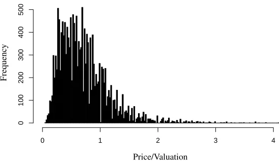
Clearly, it is not meaningful to make a simple comparison between the reached prices. A dining chair reaching $400 might be a much better price for the seller than a sofa reaching $1000. The measure I will employ is therefore the price relative to the valuation made by Laurtiz.com. In other words, if one auctions ends up with a higher Price/Valuation (P/V) ratio than another it indicates a relatively higher price. Although valuation is a good proxy for the relative attractiveness of the product, it is not enough if we want to make a fair comparison between auctions. Some items are in thin markets and risk being sold at very low prices no matter the auction development. Some items are more common and popular and therefore more con-sistently priced. And some products are just worth much more than Laurtitz.com initially expected and sold at a large premium compared to the valuation. As a result there is a huge variation in the P/V as Figure 1 shows.

You could argue that we actually do not need to make a fair comparison between single auctions as we are just interested in the average effect of timing. Yet, there is most likely a correlation between the relative popularity of an item and the bid-ding pattern of that auction. You could for instance expect more bidbid-ding wars right before expiration if more bidders are interested in an item. A certain effect of price pattern could therefore in reality be a result of popularity. To rule out this possibil-ity, the statistical analysis must somehow control for the underlying popularity on the market.

0 1 2 3 4

0

100

200

300

400

500

Price/Valuation

F

re

q

u

en

cy

Figure 1: Number of auctions with a certain P/V ratio

between the number of bidders (N) and the P/V ratio. An extra bidder does for instance result in a price increase of 6.5% on average9. The major problem is, however, that the number of bidders cannot be used as a controlling variable as this variable is endogenous. As an example, consider the effect of a certain reserve price (sometimes called the minimum price or starting bid). A high reserve price will most likely reduce the number of bidders, since the bidders with a willingness to pay below the reserve price naturally will not come forward with a bid. The direct effect of a higher reserve price is therefore fewer bidders on average. The auctions here do not have a reserve price, but the same problem will appear if the price in one auction increases fast compared to other auctions10. In fact, as scarring off bidders is one of the possible effects of the bid early strategy, it is crucial not to ignore this endogeneity problem.

An alternative proxy for popularity that does not have this endogeneity problem is the initial number of bidders11. To equalize between e.g. morning, I define initial bidders as the number of bidders the first 24 hours, denotedN24h. Although this may not be as good a proxy for market interest as the total number of bidders, it still does hint at the underlying interest amongst potential costumers12. Also, it does seem to be a reasonable proxy as the correlation betweenN24handNis 0.69. Thus,N_i24hwill be used as a control for “attractiveness” for auctioni.

To conclude, an auction with a high price is defined as an auction with a relative

9_{The result of a simple least squared regression with P/V as a response of the Number of bidders} 10_{Assuming that bidding is distributed during the auction week.}

11_{Alternatively, it could also be the number of bids or/and the initial price increase, but this might} say more about bidding strategies than of underlying interest.

high Price/Valuation ratio compared to other auctions with, in principle: 1) the sameN24h), 2) the same Valuation (V) and 3) the same values for other controls denotedX, like the time of day and the day of week. More precisely, the analysis in this paper will be based on least squared regression with a structure of Equation (1).

Pi/Vi= f(PricePatterni) +g(Ni24h,Vi, Xi) +εi

whereε_iare i.i.d. (1) The exact specification of the controls,g(), can be found in Appendix A. Moreover

g()will stay unchanged throughout, whereas the effect of price patterns, material-ized in the function f(), will be separated and analyzed.

4

Timing effects

The 17,076 auctions contain roughly 353,000 unique bids from 30,600 individual bidders. The objective here is to convert this micro-level data into some standard-ized testable characteristics at the auction (macro) level in order to link auction-level price effects to micro-auction-level bidding. Hence, the idea is to define and discuss the effect of the function f()from equation (1).

4.1 Price Jumps

As mentioned, one could have the strategy to scare off other bidders by driving up the price early, i.e. a so-called jump bid (if successful). The other strategy of particular interest is that of late bidding. A straightforward way of categorizing auctions with these strategies is to look for price jumps early and late in the auc-tion. Yet, an absolute jump in the price does not necessarily reveal anything about a strategy. A price increase of $100 could be a large increase for something inex-pensive, but a small increase for something expensive. Of course, you could be a bit more sophisticated and define a jump as a certain percentage of the valuation, but as the valuation is imperfect the basic problem remains.

What is relevant is thedistributionof the actual price increases. A bidder deciding on a strategy will basicallyeitherbid noworwait. Thus, if much of the total price increase happens early in the auction some key bidders must actively have chosen to bid earlyrather than to wait13. On the other hand, if key bidders wait and use late bidding a large proportion of the total price increase must happen during the

last hours or even minutes. Until that point the price will therefore be relatively low compared to the final price. The relevant measure of strategies must therefore be price jumps relative to the entire price increase. The first categorizations of price patterns (and thus the underlying bidding strategies) is a number of binary variables defined as:

jumpitsmall =

1,if the price increase for auction i at timetis 40% - 50% of the total

0,else

jumpitlarge=

1,if the price increase for auction i at timetis>50% of the total

0,else

These jumps are defined fort={1,2, ...,9}, where

t=1 is defined as Day 1 (the first 24 hours)

t=2 is defined as Day 2 (24h to 48h) ...

t=6 is Day 6 until 2.a.m.

t=7 is Day 7 until 3 hours before the end

t=8 is -3 hours until -15 minutes (-3h)

t=9 is the last 15 minutes (-15min)

I did not take into account any of the 3 minutes extensions of the soft ending which implies that if an auction was extended 2 x 3 minutes,t=9 will be the last 9 min-utes of the ordinary auction time and 6 minmin-utes of extended time. The size of jumps and the time intervals are of course rather arbitrary, but chosen to get a reasonable number of auctions within each group without loosing the link to the strategies. The exact proportion of auctions in each group is specified in Appendix A, but the overall levels are:

34.4% does not have any jumps 25.3% has a small jump 35.2% has a large jump 2.7% has two small jumps

2.3% has a small and a large jump.

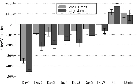
It turns out that the effect of such price jumps is surprisingly clear and consistent. Figure 2 shows the estimates and 95% confidence intervals from regressing the Price/Valuation ratio against these binary jump variables, i.e. a least squares re-gression similar to that of Equation (1). The exact specification and results can be seen in Appendix A.3.

Small Jumps Large Jumps

P

ri

ce

/V

al

u

at

io

n 0

-50% -40% -30% -20% -10% +10% +20%

Day1 Day2 Day3 Day4 Day5 Day6 Day7 -3h -15min

Figure 2: Average effect on P/V from price jumps

as early as possible and try to make the price jump.

4.2 Price Increase Distributions

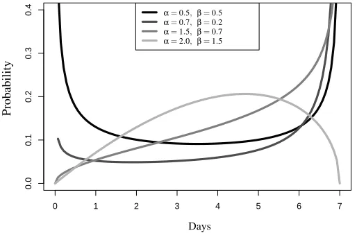
While the price jumps and the time intervals may seem arbitrary, another approach is to look directly at the distribution of price increases. Again, we have in principle 17,076 different distributions, but many do share some characteristics. Fitting a relative simple parametric function is therefore a feasible approach. In particular, it seems reasonable to look among probability distribution functions as probability distributions and price increase distribution would naturally share some character-istics (Price start in zero and end up at 100% of the final price – much like a cumu-lative probability distribution). The challenge is to find a probability distribution function which is both flexible and possible to interpret with respect to strategies.

Among the hyperlinks at Lauritz.com’s front page there is one for “New items” and one for “Last Chance”. This, together with the bid early or late strategies, could lead to a over-representation of bids the first and last day, and if you look further into the data this is in fact the case. 19% of all the unique bids arrive the first day and 46% the last day14. As a consequence, the potential density function needs to be able to take a sort of U-shape. Still, the bidding can of course also be characterized by more complex patterns. The potential density function must therefore also be able to take other shapes like an inverted U.

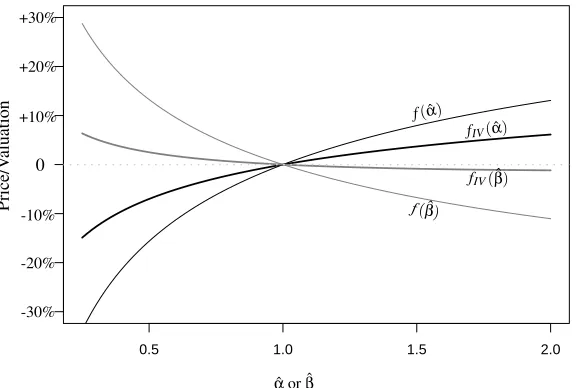
One density function which can contain most such bidding patterns in a simple

manner is the Beta distribution function. Furthermore, the two parameters (αand

β) of the Beta distribution are easy to interpret in relation to the bid early or late strategies. To illustrate, consider the different specifications of a Beta probability density function in Figure 3. αis directly linked to the proportion of early price increases, andβto the late price increases. The lower the parameters, the higher the proportion of price increases. Whenα=β=1 it is a uniform distribution and ifα<1 andβ<1, the distribution has a U-shape with a high proportion of price increases early and late.

0 1 2 3 4 5 6 7

0.0

0.1

0.2

0.3

0.4

P

ro

b

ab

il

it

y

α=0.5, β=0.5

α=0.7, β=0.2

α=1.5, β=0.7

α=2.0, β=1.5

Days

Figure 3: Beta distributions

It is relatively simple to estimateαandβfor every auction as this can be done from the empirical mean and variance with the method-of-moments (see Appendix A.2). The result of this estimation is that 60.6% of the auctions have estimates ofαand

βwhere they both are below 1, and only 19.6% where they both are above. Thus, as expected most auctions are estimated to have U-shape distributions of bidding. Figure 4 shows the estimated effects of ˆαand ˆβon the Price/Valuation ratio. They are found in a regression similar to that of section 4.1, but where the function f()

from Equation (1) is defined as:

f() =a11·ln(αˆi) +a12·ln(αˆi)2+a21·ln(βˆi) +a22·ln(βˆi)2

The figure shows a clear negative effect of higher ˆβ and a clear positive effect of higher ˆα. Furthermore, the estimated parameters, a11,a12,a21,a22 are highly

significant which also can be seen from the 95% confidence intervals shown with the broken lines (very close to the estimate). In fact, this model with only two variables describing the price pattern, seems to be a much better model than that in section 4.1, as it increases the adjustedR2with 0.08 to 0.34. The full results of the regression can be found in Appendix A.3.

0.5 1.0 1.5 2.0

P

ri

ce

/V

al

u

at

io

n f(_αˆ)

f(_βˆ₎

ˆ

αor ˆβ

0

-10%

-20%

-30% +30%

+20%

+10%

Figure 4: Effect on P/V of estimatedαandβ

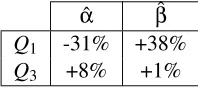
a lower proportion of price increases in the beginning of auction. In other words, the more price increases in the beginning (lower ˆα), the lower the average prices. For ˆβthe effect is the opposite; The higher the proportion of price increases late in the auction (lower ˆβ), the higher the average price. To further quantify, consider the estimated effects of the lower (Q1) and upper quartile (Q1) for ˆαand ˆβin Table

115_{. Basically, both the sign and the magnitude supports the effects found from}

price jumps.

ˆ

α _βˆ

Q1 -31% +38%

Q3 +8% +1%

Table 1: Quantifying the effect of ˆαand ˆβ

5

Instrumental Variable Regression

One possible explanation for these results is that early price increase scare off bid-ders. As argued, this was one of the reasons for using N24hinstead of total N to control for popularity. To dig a little deeper, it is therefore natural to look at the indirect effect which price jumps have on totalN. This is easily done by replacing

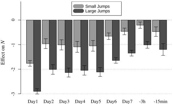
P/V with N as the dependent variable in the first regression of section 4.1. The result of this OLS regression can be found in Appendix B, but the main results are shown in Figure 5.

15_{The values for these quartiles are:Q}αˆ

1 =0.28,Qα3ˆ =1.49,Q ˆ

β

1=0.17, andQ ˆ

β

Small Jumps Large Jumps

0

-1

-2

-3

Day1 Day2 Day3 Day4 Day5 Day6 Day7 -3h -15min

E

ff

ec

t

o

n

N

Figure 5: Indirect effect on Number of bidders

As shown, all jumps have a negative effect on the total number of bidders entering the auction. Also, large and early jumps are more efficient to reduce entry. How-ever, this is as expected as a higher price naturally would deter some bidders from entering. The question is if this effect is powerful enough to be the driving factor. To answer this question, the last step must be to isolate the direct effect of price jumps on prices. In other words, if the indirect effect of reduced entry is taken into account, what is the remaining effect of jumps on prices?

Such an analysis can be performed as Instrumental Variable (IV) regression using a two stage least square procedure. The first step in this procedure is to predict totalNon the basis of jumps,N24hand other controls. This is the regression from above. This predictedNis then used as exogenous variable in the next regression where P/V is the dependent variable.

In theory, the two regression must be estimated simultaneously as the error terms will be correlated16. Traditionally, this procedure is therefore represented as a sys-tems of equations as shown in Equation (2), whereN24his said to be the instrument forN.

Pi/Vi= f(jumpsi) +g(Ni,Vi,zi) +εi

Ni= f(jumpsi) +g(Ni24h,Vi, zi) +νi

(2)

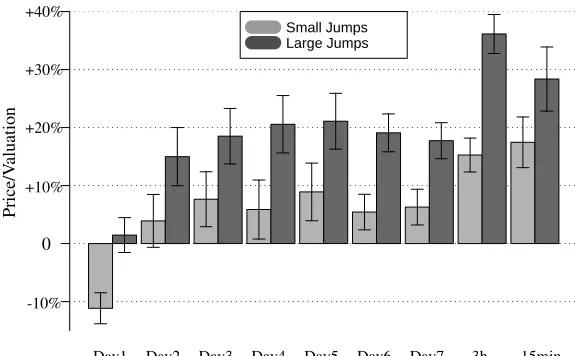
The result of this IV regression shows that the direct (intrinsic) effects of jumps on prices are generally positive as shown in Figure 617. This is more the case the larger

16_{In practice they are however estimated in a two step procedure, but where the error terms are} adjusted subsequently

and later the jumps are. In itself a price jump will therefore most likely contribute to higher prices perhaps as a sort of momentum effect in the short run.

To conclude, price jumps have a positive intrinsic effect, but because they also scare off bidders this effect can be reversed. The surprising part is, however, that the deterrence effect is often so strong that the positive intrinsic effect is likely to be reversed. Naturally this is more the case the sooner the price jump, but the deterrence effect is in fact so strong that up until the last 3 hours, it will dominate on average.

Small Jumps Large Jumps

P

ri

ce

/V

al

u

at

io

n

0

+40%

+30%

-10% +10% +20%

Day1 Day2 Day3 Day4 Day5 Day6 Day7 -3h -15min

Figure 6: Intrinsic effect of price jumps (IV regression)

This analysis can similarly be performed with the estimated parameters from the Beta distribution of section 4.2. Instead of analyzing the effect of ˆα and ˆβ on the total number of bidders, I will go directly to the Instrumental variable (IV) regression. The result of this (IV) regression can be found in Figure 718. Here the effect of IV estimates are shown on top of the estimates from section 4.2. Clearly, this shows that removing the deterrence effect on bidders does moderate the effect of early and late bidding (low ˆαand ˆβ), but the effect is not reversed as in the case of jumps.

The overall conclusion is that early price increases on average always will scare off bidders. Price jumps may scare off more bidders, but will perhaps also lead to a momentum effect and have a positive intrinsic effect on the price. But since a bidder cannot control how other bidders bid up the price, the important conclu-sion is that an early bid, whether this leads to slow or fast early price increases, unambiguously is the best strategy.

The advice for later entry is on the other hand always to try to jump the price. Late

0.5 1.0 1.5 2.0

P

ri

ce

/V

al

u

at

io

n _f(αˆ)

f(_βˆ₎

fIV(αˆ)

fIV(βˆ)

ˆ

αor ˆβ

0

-10%

-20%

-30% +30%

+20%

+10%

Figure 7: Effect on P/V (IV estimation)

price increase will no matter the size intrinsically lead to higher prices, perhaps because the relative low price will always attract potential bidders19. Yet a price jump will on average also later on prevent some of these potential late bidders from entering, and the net effect on the final price from late jumps is therefore less positive than a more slow, but also late price increases.

6

Discussion

The analysis in this article suggests that the timing of bids does matter, and unlike the prototypical behavior it seems to be a dominating strategy to bid sooner rather than later. Although both approaches (jumps and the Beta distributions) might seem a little artificial, I do believe that the combination makes a strong argument. There is, however, one possible critique; the potential endogeneity of (N24h). Prin-cipally, both jumps day 1 and ˆαdo influenceN24hin the same way that the general price pattern makes totalNendogenous. Yet, if we follow this logic, the effect of a price increase on day 1 must in fact be even more negative, had theN24hnot been negatively influenced by that early price increase. Hence, this argument will only make the conclusion stronger.

Generally, you could also have doubts about the effectiveness of the controlling variables. In principal there could still be some unobserved variables, e.g. lower quality, which is the real explanation behind the lower price of auctions with early

price increases. However, auctions with much of the price increase early do gener-ally have more initial bidders than the average auction. Thus, this does not indicate lower quality, rather the opposite, so perhaps the deterrence effect is even stronger than estimated here. Again, this could make the conclusion stronger rather than weaker.

In a broader perspective these results basically tell us that the entry threshold is often different from the final bid. Hence bidders must change their willingness to pay during the auction. That is in itself not too surprising as other analysis on eBay data have had the same insinuation20. This analysis does, however, give a little more insight into how this change in preference is triggered. It seems to be coursed by either the relative low price or the momentum in the price increase. Let me take each case separately.

The positive intrinsic effect of price jumps cf. Figure 6 could suggest some mo-mentum in the bidding. Once the price starts to increase, bidders might get excited and competitive. Ariely and Simonsohn (Forthcomming) e.g. show that auctions with a low reserve, and hence many bidders/bids, have a higher probability of receiving more bids than similar auctions with a higher reserve price and fewer bidders/bids.

This kind of competitive behavior might even turn into “auction fever” where bid-ders get carried away by the idea of winning, see e.g. Lee and Malmendier (2006) or Ariely and Simonsen (2003). However, auctions with late jumps (auctions with a high likelihood of “auction fever”) have a lower probability of return21_{. Thus,}

bidders who won the item in a very competitive auction will less often take ad-vantage of the 14 days right to return as provided by the auction house. “Auction fever” does therefore not seem to be a dominating explanation.

The other explanation is that bidders seem to be attracted by the “good deal” and once they have entered they get caught. This could therefore be an example of the so-called pseudo- or quasi-endowment effect as suggested by e.g. Ariely et al. (2004) and Wolf et al. (2005). Basically, the idea is that bidders get used to the idea of buying and will therefore be willing to increase their bids in order to avoid the loss of this pseudo-endowment.

The results here suggest that this effect is especially pronounced when prices are relative low and bidders get overoptimistic about their possibility to win. In other words, it is when bidders expect to win with a high probability that they feel owner-ship and get caught in the auction. This analysis does in fact suggests that bidders either create this feeling of ownership very fast or create it before entering e.g.

dur-20_{see e.g. Ariely et al. (2004), Ariely and Simonsohn (Forthcomming), Ku et al. (2005), or Wolf} et al. (2005).

ing observation. However, these conclusion are still on a very speculative level so this is an obvious area for further research.

References

Ariely, D., Heyman, J. and Orhun, Y.: 2004, Auction fever: The effect of oppo-nents and the quasi-endowment on product valuations, Journal of Interactive Marketing18(4).

Ariely, D. and Simonsen, I.: 2003, Buying, bidding, playing or competing? value assessment and decision dynamics in online auctions,Journal of Consumer Psy-chology13, 113–123.

Ariely, D. and Simonsohn, U.: Forthcomming, When rational sellers face non-rational consumers: Evidence from herding on ebay,Management Science. Bajari, P. and Hortacsu, A.: 2003, The winner’s curse, reserve prices, and

endoge-nous entry: empirical insights from ebay auctions,RAND Journal of Economics

34(2), 329–355.

Bajari, P. and Hortacsu, A.: 2004, Economic insights from internet auctions, Jour-nal of Economic LitteratureXLII, 457–486.

Hou, J.: 2007, Late bidding and the auction price: evidence from ebay,Journal of Product & Brand Management16, 422–428.

Ku, G., Malhotra, D. and Murnighan, J. K.: 2005, Towards a competitive arousal model of decision-making: A study of auction fever in live and internet auctions,

Organizational Behavior and Human Decision Processes96(2), 89–103. Lee, H. and Malmendier, U.: 2006, The bidder’s curse, Working Paper, Stanford

University.

Ockenfels, A. and Roth, A. E.: 2002, The timing of bids in internet auctionsmarket design, bidder behavior, and artificial agents,AI Magazine23(3), 79–87. Ockenfels, A. and Roth, A. E.: 2006, Late and multiple bidding in second price

internet auctions: Theory and evidence concerning different rules for ending an auction,Games and Economic Behavior55(2), 297–320.

Roth, A. E. and Ockenfels, A.: 2002, Last-minute bidding and the rules for ending second-price auctions: Evidence from ebay and amazon auctions on the internet,

American Economic Review92(4), 1093–1103.

APPENDIX

A

Basic regressions behind Timing Effects

The main results of this paper, i.e. the effects on the Price/Valuation (P/V) ratio of section 4, is based on a simple Ordinary Least Squared (OLS) regression. As discussed in section 3, the controlling variables is of great importance to the relia-bility of the result. I have therefore used all available controls without considering significance level. With the large amount of degrees of freedom there is no need to reduce the model as much as possible. The controlling variables are therefore:

Initial bidders the first 24 hours (N24h) As discussed, the most important con-trolling variable in the basic regression is the initial bidders as a proxy for underlying interest. Besides a linear term there is also a quadratic and a cubic term as they are also significant.

Valuation Even though valuation is also used to define the dependent variable (P/V), valuation is also in itself an important explanatory variable. Further-more, the interaction between Valuation andN24his also significant.

Hour Auctions finish throughout the day from 8 a.m. to midnight. As some hours may be more successful than others, I therefore us this as a control.

Weekday Similarly auctions are sold throughout the week although very few on Sundays.

Month Wintertime is more busy and, as it turns out, more successful in getting higher prices.

Category As mentioned, 71% of the auctions are in the “Table and chairs” and 29% are in the “miscellaneous” group. I also use these categories as controls.

A.1 Jumps

The first regression uses price jumps as dummy variables as a categorization of the price structure. In section 4.1 includes the reasoning and definition of these jumps. The exact sizes of the jumps are of course a bit arbitrary, but they are principal chosen to get a even distribution of the auctions. The percentage of auctions with a certain jump is listed in Table 1.

A.2 The Beta distribution

The second regression utilizes the Beta distribution to describe the price pattern. The probability density function of the beta distribution is defined as:

f(x;α,β) = xα

−1_(1−x)β−1

R1

0 uα−1(1−u)β−1du

I use the method-of-moments estimates of the two parameters in the beta distribu-tion. In other words ˆα and ˆβare calculated from the empirical mean, ¯x, and the empirical variance,v, as:

ˆ

α=x¯

_¯

x(1−x¯)

v −1

and βˆ = (1−x¯)x¯(1_v−x¯)−1

A.3 Results

Regression 1: Regression 2: Jumps Beta distribution

Estimate Std. Error Estimate Std. Error

Intercept 0.8348 0.1243 *** 0.6455 0.1176 ***

jump1 0.4-0.5 -0.3507 0.0126 *** - -jump2 0.4-0.5 -0.0883 0.0213 *** - -jump3 0.4-0.5 -0.0725 0.0221 ** - -jump4 0.4-0.5 -0.1047 0.0237 *** - -jump5 0.4-0.5 -0.0653 0.0232 ** - -jump6 0.4-0.5 -0.0465 0.0142 ** -

-jump7 0.4-0.5 -0.0079 0.0144 -

-jump3h 0.4-0.5 0.1134 0.0137 *** - -jump15min 0.4-0.5 0.1038 0.0206 *** -

-jump1>0.5 -0.4546 0.0114 *** - -jump2>0.5 -0.2131 0.0209 *** - -jump3>0.5 -0.1955 0.0194 *** - -jump4>0.5 -0.1563 0.0207 *** - -jump5>0.5 -0.1795 0.0192 *** - -jump6>0.5 -0.1092 0.012 *** - -jump7>0.5 -0.0637 0.0125 *** - -jump3h>0.5 0.1705 0.0144 *** - -jump15min>0.5 0.0849 0.0255 *** -

-a11: ln(αˆ) - - 0.2070 0.0035 *** a12: ln(αˆ)2 - - -0.0264 0.0005 *** a21: ln(βˆ) - - -0.1753 0.0032 *** a22: ln(βˆ)2 - - 0.0232 0.0007 ***

Valuation -0.0001 0.0000 *** -0.0001 0.0000 ***

N24h _{0.2146 0.0074 *** 0.2820 0.0079 ***}

Continued from previous page

Estimate Std. Error Estimate Std. Error

(N24h)2 _{-0.0257 0.0023 *** -0.0376 0.0024 ***} (N24h)3 _{0.0011 0.0002 *** 0.0016 0.0002 ***}

Valuation*N24h _{0.0000 0.0000 *** 0.0000 0.0000 ***}

factor(Category)Modern furniture - tables and chairs 0.0021 0.0066 0.0184 0.0062 **

factor(Month)2 0.0038 0.0167 0.0028 0.0158 factor(Month)3 -0.0599 0.0171 *** -0.0568 0.0162 *** factor(Month)4 -0.0797 0.0167 *** -0.0761 0.0158 *** factor(Month)5 -0.0804 0.0163 *** -0.0796 0.0154 *** factor(Month)6 -0.0948 0.0162 *** -0.0957 0.0153 *** factor(Month)7 -0.0970 0.0183 *** -0.1061 0.0173 *** factor(Month)8 -0.0750 0.0163 *** -0.0728 0.0154 *** factor(Month)9 -0.1055 0.0157 *** -0.1118 0.0149 *** factor(Month)10 -0.0766 0.0165 *** -0.0808 0.0156 *** factor(Month)11 -0.0962 0.0162 *** -0.0990 0.0153 *** factor(Month)12 -0.0860 0.0170 *** -0.0919 0.0160 ***

factor(Ends weekday)2 -0.0097 0.0091 -0.0151 0.0086 . factor(Ends weekday)3 -0.0084 0.0092 -0.0202 0.0087 * factor(Ends weekday)4 -0.0116 0.0097 -0.0223 0.0092 * factor(Ends weekday)5 0.0002 0.0097 -0.0133 0.0092 factor(Ends weekday)6 -0.0626 0.0449 -0.0601 0.0426 factor(Ends weekday)7 0.0062 0.1947 -0.0234 0.1844

factor(Time of day)8 -0.0866 0.1264 -0.0957 0.1197 factor(Time of day)9 -0.0706 0.1242 -0.0794 0.1176 factor(Time of day)10 -0.0446 0.1238 -0.0588 0.1172 factor(Time of day)11 -0.0428 0.1236 -0.0443 0.1170 factor(Time of day)12 -0.0422 0.1235 -0.0444 0.1169 factor(Time of day)13 -0.0432 0.1234 -0.0519 0.1168 factor(Time of day)14 -0.0472 0.1233 -0.0601 0.1168 factor(Time of day)15 -0.0574 0.1233 -0.0646 0.1168 factor(Time of day)16 -0.0551 0.1235 -0.0690 0.1170 factor(Time of day)17 -0.0314 0.1237 -0.0488 0.1172 factor(Time of day)18 -0.0395 0.1286 -0.0579 0.1218 factor(Time of day)19 -0.0223 0.1590 -0.1347 0.1505 factor(Time of day)20 -0.1654 0.1615 -0.2073 0.1529 factor(Time of day)22 -0.1609 0.4079 -0.0568 0.3865 factor(Time of day)23 -0.1765 0.1615 -0.1324 0.1529

Residual standard error: 0.3886 Residual standard error: 0.3681 on 17019 degrees of freedom on 17033 degrees of freedom Significant codes: *** 0.001, ** 0.01, * 0.05 AdjustedR2: 0.2642 AdjustedR2: 0.3396

Table 2: Effects on the Price/Valuation ratio

B

Effect of jumps on total

N

Estimate Std. Error

Intercept 4.6810 0.5927 ***

jump1 0.4-0.5 -1.7620 0.0600 *** jump2 0.4-0.5 -0.9605 0.1017 *** jump3 0.4-0.5 -1.0100 0.1054 *** jump4 0.4-0.5 -1.0920 0.1130 *** jump5 0.4-0.5 -1.0510 0.1105 *** jump6 0.4-0.5 -0.6581 0.0676 *** jump7 0.4-0.5 -0.4633 0.0686 *** jump3h 0.4-0.5 -0.2088 0.0654 ** jump15min 0.4-0.5 -0.4712 0.0982 ***

jump1>0.5 -2.9020 0.0546 *** jump2>0.5 -2.0120 0.0995 *** jump3>0.5 -2.1370 0.0925 *** jump4>0.5 -2.0480 0.0986 *** jump5>0.5 -2.1140 0.0915 *** jump6>0.5 -1.6440 0.0571 *** jump7>0.5 -1.3470 0.0595 *** jump3h>0.5 -1.0120 0.0688 *** jump15min>0.5 -1.1990 0.1215 ***

Valuation 0.0005 0.0000 ***

N24h 1.0830 0.0352 ***

(N24h)2 _{0.0267 0.0110 *} (N24h)3 _{0.0004 0.0009}

Valuation*N24h -0.0001 0.0000 ***

factor(Category)Modern furniture - tables and chairs 0.2421 0.0314 ***

factor(Month)2 -0.0198 0.0794 factor(Month)3 -0.1365 0.0814 factor(Month)4 -0.2971 0.0796 *** factor(Month)5 -0.3675 0.0776 *** factor(Month)6 -0.4599 0.0771 *** factor(Month)7 -0.2808 0.0873 ** factor(Month)8 -0.3541 0.0779 *** factor(Month)9 -0.2022 0.0749 ** factor(Month)10 0.0735 0.0787 factor(Month)11 -0.0624 0.0773 factor(Month)12 -0.0278 0.0808

factor(Ends weekday)2 -0.0342 0.0433 factor(Ends weekday)3 -0.0804 0.0436 factor(Ends weekday)4 -0.1110 0.0461 * factor(Ends weekday)5 0.0462 0.0463 factor(Ends weekday)6 0.0990 0.2143 factor(Ends weekday)7 1.4190 0.9285

factor(Time of day)8 -0.2703 0.6026 factor(Time of day)9 -0.2400 0.5924 factor(Time of day)10 -0.0556 0.5902 factor(Time of day)11 -0.1374 0.5895 factor(Time of day)12 -0.1883 0.5888 factor(Time of day)13 -0.2218 0.5883 factor(Time of day)14 -0.2795 0.5881 factor(Time of day)15 -0.4160 0.5883 factor(Time of day)16 -0.4533 0.5891

Continued from previous page

Estimate Std. Error

factor(Time of day)17 -0.3317 0.5902 factor(Time of day)18 -0.1886 0.6133 factor(Time of day)19 -0.2950 0.7582 factor(Time of day)20 -1.4090 0.7701 factor(Time of day)22 0.4511 1.9450 factor(Time of day)23 -0.4437 0.7700

Residual standard error: 1.853 on 17019 degrees of freedom, AdjustedR2: 0.6357 Significant codes: *** 0.001, ** 0.01, * 0.05

Table 3: Effect on final number of bidders

C

Instrumental Variable Regression

As described in section 5, Instrumental Variable (IV) Regression can isolate the direct effects of the price pattern, i.e. disregard the indirect effect on the entry of new bidders and only see the direct effect on prices. The results of this IV regression, i.e. the direct effect on P/V, is listed in Table 5 below using both jumps and the Beta distribution to describe the price pattern.

IV Regression: IV Regression: Jumps Beta distribution

Estimate Std. Error Estimate Std. Error

Intercept -0.4160 0.1520 ** -0.6961 0.1692 ***

jump1 0.4-0.5 -0.1120 0.0136 *** -

-jump2 0.4-0.5 0.0391 0.0233 -

-jump3 0.4-0.5 0.0764 0.0242 ** - -jump4 0.4-0.5 0.0587 0.0260 * - -jump5 0.4-0.5 0.0891 0.0254 *** - -jump6 0.4-0.5 0.0544 0.0156 *** - -jump7 0.4-0.5 0.0629 0.0157 *** - -jump3h 0.4-0.5 0.1530 0.0149 *** - -jump15min 0.4-0.5 0.1750 0.0223 *** -

-jump1>0.5 0.0147 0.0153 -

-jump2>0.5 0.1500 0.0256 *** - -jump3>0.5 0.1850 0.0244 *** - -jump4>0.5 0.2060 0.0252 *** - -jump5>0.5 0.2110 0.0246 *** - -jump6>0.5 0.1910 0.0167 *** - -jump7>0.5 0.1770 0.0158 *** - -jump3h>0.5 0.3610 0.0171 *** - -jump15min>0.5 0.2840 0.0282 *** -

-a11: ln(αˆ) - - 0.0948 0.0035 *** a12: ln(αˆ)2 - - -0.0092 0.0007 *** a21: ln(βˆ) - - -0.0266 0.0049 ***

Continued from previous page

Estimate Std. Error Estimate Std. Error

a22: ln(βˆ)2 - - 0.0139 0.0009 ***

Valuation -0.0002 0.0000 *** -0.0003 0.0000 ***

N24h 0.4280 0.0309 *** 0.5809 0.0410 ***

(N24h)2 _{-0.0303 0.0036 *** -0.0460 0.0047 ***} (N24h)3 _{0.0006 0.0001 *** 0.0010 0.0002 ***}

Valuation*N24h _{0.0000 0.0000 *** 0.0000 0.0000 ***}

factor(Category)Modern furniture - tables and chairs -0.0282 0.0072 *** -0.0349 0.0077 ***

factor(Month)2 0.0049 0.0179 0.0224 0.0192 factor(Month)3 -0.0424 0.0184 * -0.0212 0.0197 factor(Month)4 -0.0344 0.0180 -0.0073 0.0193 factor(Month)5 -0.0301 0.0176 0.0036 0.0188 factor(Month)6 -0.0236 0.0175 0.0168 0.0188 factor(Month)7 -0.0464 0.0198 * -0.0144 0.0212 factor(Month)8 -0.0290 0.0176 0.0025 0.0189 factor(Month)9 -0.0700 0.0170 *** -0.0361 0.0182 * factor(Month)10 -0.0808 0.0178 *** -0.0571 0.0190 ** factor(Month)11 -0.0799 0.0174 *** -0.0467 0.0187 * factor(Month)12 -0.0759 0.0182 *** -0.0376 0.0196

factor(Ends weekday)2 -0.0023 0.0098 0.0022 0.0105 factor(Ends weekday)3 0.0029 0.0099 0.0100 0.0106 factor(Ends weekday)4 0.0008 0.0104 0.0053 0.0111 factor(Ends weekday)5 -0.0052 0.0104 -0.0038 0.0112 factor(Ends weekday)6 -0.0692 0.0484 -0.1104 0.0517 factor(Ends weekday)7 -0.2970 0.2100 -0.3787 0.2240

factor(Time of day)8 -0.0735 0.1360 -0.0633 0.1453 factor(Time of day)9 -0.0684 0.1340 -0.0852 0.1429 factor(Time of day)10 -0.0702 0.1330 -0.0953 0.1424 factor(Time of day)11 -0.0576 0.1330 -0.0770 0.1422 factor(Time of day)12 -0.0536 0.1330 -0.0761 0.1421 factor(Time of day)13 -0.0495 0.1330 -0.0646 0.1419 factor(Time of day)14 -0.0404 0.1330 -0.0548 0.1418 factor(Time of day)15 -0.0340 0.1330 -0.0407 0.1419 factor(Time of day)16 -0.0170 0.1330 -0.0245 0.1421 factor(Time of day)17 -0.0283 0.1330 -0.0363 0.1423 factor(Time of day)18 -0.0267 0.1390 -0.0261 0.1479 factor(Time of day)19 -0.0090 0.1710 -0.0544 0.1830 factor(Time of day)20 0.0526 0.1740 0.0733 0.1858 factor(Time of day)22 -0.1060 0.4390 -0.0706 0.4698 factor(Time of day)23 -0.1600 0.1740 -0.1911 0.1857

Residual standard error: 0.4182 Residual standard error: 0.4471 Significant codes: *** 0.001, ** 0.01, * 0.05 on 17019 degrees of freedom on 17033 degrees of freedom

D

Returned

The Danish Sale of Goods Act specifies 14 days of right to return for all trade on the internet with private consumers. There has been some discussion on whether internet auctions like Lauritz.com are included in this, but for now they are. Hence, all private winners have two weeks to regret their purchase.

Naturally, Laurtiz.com is trying to discourage the use of this right to return as this may encourage reckless or perhaps even fake bidding. Also, returned items have to be put on auction again. Although this right is described on the auctions site, it may not be clear to all users. Furthermore, buyers must in principal pay for the item within 3 days while you will only get your money back within a 30 days period.

Here, I have modeled the actual return as logit regression in order to find the factors that have a positive or negative influence on the probability to return. The result of this logit regression is listed in Table 6 below.

Estimate Std. Error

(Intercept) -5.8920 1.1840 ***

jump1 0.4-0.5 0.0095 0.1375 jump2 0.4-0.5 0.6969 0.1887 *** jump3 0.4-0.5 -0.0049 0.2441 jump4 0.4-0.5 0.1401 0.2454 jump5 0.4-0.5 0.1495 0.2520 jump6 0.4-0.5 -0.0290 0.1602 jump7 0.4-0.5 -0.3257 0.1825 . jump3h 0.4-0.5 -0.0635 0.1496 jump15min 0.4-0.5 -0.3136 0.2546

jump1>0.5 0.2330 0.1221 . jump2>0.5 0.2777 0.2134 jump3>0.5 0.5374 0.1861 ** jump4>0.5 0.4896 0.2053 * jump5>0.5 0.4939 0.1880 ** jump6>0.5 0.1646 0.1279 jump7>0.5 0.2457 0.1295 . jump3h>0.5 0.1449 0.1490 jump15min>0.5 -0.0558 0.2941

Valuation 0.0001 0.0000 ***

N 0.0765 0.0178 ***

Valuation*N 0.0000 0.0000 **

factor(Category)Modern furniture - tables and chairs -0.0184 0.0702

factor(Month)2 -1.8220 1.1190 factor(Month)3 1.6130 0.5380 ** factor(Month)4 2.3740 0.5181 *** factor(Month)5 2.7420 0.5120 *** factor(Month)6 2.9270 0.5104 *** factor(Month)7 3.0530 0.5158 ***

Continued from previous page

Estimate Std. Error

factor(Month)8 3.0070 0.5102 *** factor(Month)9 3.1580 0.5077 *** factor(Month)10 3.2130 0.5093 *** factor(Month)11 3.0860 0.5094 *** factor(Month)12 3.2170 0.5104 ***

factor(Ends weekday)2 -0.0414 0.0978 factor(Ends weekday)3 -0.0153 0.0975 factor(Ends weekday)4 0.0473 0.1003 factor(Ends weekday)5 0.0392 0.1006 factor(Ends weekday)6 -0.0019 0.4747 factor(Ends weekday)7 -10.0600 155.2000

factor(Time of day)8 -0.1953 1.1020 factor(Time of day)9 0.1373 1.0710 factor(Time of day)10 -0.1845 1.0670 factor(Time of day)11 -0.1160 1.0650 factor(Time of day)12 -0.1840 1.0630 factor(Time of day)13 -0.1515 1.0620 factor(Time of day)14 -0.4162 1.0620 factor(Time of day)15 -0.3470 1.0620 factor(Time of day)16 -0.3732 1.0650 factor(Time of day)17 -0.6352 1.0700 factor(Time of day)18 0.0914 1.1180 factor(Time of day)19 -0.0796 1.4990 factor(Time of day)20 -0.6189 1.5010 factor(Time of day)22 14.8000 324.7000 factor(Time of day)23 -0.3891 1.4880

Residual deviance: 7696.9 on 17021 degrees of freedom Significant codes: *** 0.001, ** 0.01, * 0.05