Rough Set Approach for the Classification of
Advertisement in the Development of Business
Establishment
Sujogya Mishra
Research Scholar,Utkal University Bhubaneswar-751004, India
Shakti Prasad Mohanty
Department of Mathematics College of Engineering andTechnology
Bhubaneswar-751003, India
Sateesh Kumar Pradhan
Department of ComputerScience Utkal University Bhubaneswar-751004, India
ABSTRACT
In the current age business establishments are basically depends upon advertisement to attain success . In this paper we consider different forms of advertisements then using rough set concept, we find the best possible forms of advertisement. To develop this concept we consider 1000 samples initially and applying correlation techniques the number reduces to 20 which appears to be dissimilar with respect to advertisements initially. We classified the entire paper in to four section , section 1 deals with the literature review and in the section 2 deals with the experiment on the data which we collected from different sources and in last two section deals with the algorithm which we develop using rough set concept and validation of the algorithm using statistical test .
Keywords
Rough Set Theory, business data, Granular computing, Data mining
1.INTRODUCTION
The rising demand for business and wide use of internet for the growth of business resulted in huge data generation in manifold ways. The data so generated not only confuses the mind of the user but also it creates problem to derive the useful data for the application of the user. This has posed an obvious challenge for the researchers to develop methods to reduce the data set and to derive the relevant data for desired application. The application of rough set theory has an important role to play for knowledge discovery in data base(s).The ever growing field of knowledge discovery (KD) helps in extraction of hidden information from large database[3]. Data mining is also considered as essential tool in this knowledge discovery process which uses techniques from different disciplines ranging from machine learning, statistics information sciences, database, visualization ([4]-[12]). Further, prediction of business failure needs a systematic and scientific study. The first approach to predict business failure started in 1995 by Zopounidis( [24]-[26]). The methods proposed are the “five C” methods, the “LAPP” method, and the “credit-men” method. Then, financial ratios methodology was developed for business failure prediction problem. This approach gives rise the methods for business failure prediction based on multivariate statistical analysis ( Altman ([13]-[15]), Beaver[17], Courtis[18]). Frydman et al[19] first employed recursive et al[16], multi-factor model by Vermeulen et al[23] are also other methods developed for business failure prediction.
This paper presents a methodology for business success by reduction of attributes using rough set theory, portioning, while Gupta et al[20] use mathematical programming as an alternative to multivariate discriminant analysis for business failure prediction problem. Other methods used were survival analysis by Luoma, Laitinenl[21] which is a tool for company failure prediction, expert systems by Messier and Hansen[22] , neural network by Altman
2.PRILIMINARIES
2.1 Rough Set
Rough set theory as introduced by Z. Pawlak[2] is an extension of conventional set theory that support approximations in decision making.
2.1.1
Approximation Space:
An Approximation space is a pair (U , R) where U is a non-empty finite set called the universe R is an equivalence relation defined on U.
2.1.2
Information System:
An information system is a pair S = (U , A), where U is the non-empty finite set called the universe, A is the non-empty finite set of attributes
2.1.3
Decision Table:
A decision table is a special case of information systems
S= (U , A= C U {d}), where d is not in C.
Attributes in C are called conditional attributes and d is a designated attribute called the decision attribute.
2.1.4
Approximations of Sets:
Let S = (U, R) be an approximation space and X be a subset of U.
The lower approximation of X by R in S is defined as
RX = { e ε U | [e] ε X} and
The upper approximation of X by R in S is defined as
where [e] denotes the equivalence class containing e.
A subset X of U is said to be R-definable in S if and only if
¯RX= RX
A set X is rough in S if its boundary set is nonempty. }
] /[
{
e U e X
2.2 Dependency of Attributes
Let C and D be subsets of A. We say that D depends on C in a degree k (0 ≦ k ≦ 1) denoted by C →k D if
If k = 1 we say that D depends totally on C.
If k < 1 we say that D depends partially (in a degree k) on C
2.3 Dispensable and Indispensable
Attributes
Let S = (U, A = C υ D) be a decision table. Let c be an attribute in C. Attribute c is dispensable in S if POSC(D)= POS(C-{c})(D)otherwise, c is indispensable. A decision table S is independent if all attributes in C are indispensable.
Rough Set Attribute Reduction (RSAR) provides a filter based tool by which knowledge may be extracted from a domain in a concise way; retaining the information content whilst reducing the amount of knowledge involved
2.4 Reduct and Core
Let S = (U, A=C U D) be a decision table. A subset R of C is a reduct of C, if POSR(D) = POSC(D) and S’ = (U, RUD) is independent ,ie., all attributes in R are indispensible in S’. Core of C is the set of attributes shared by all reducts of C. CORE(C) = ∩RED(C) where, RED(C) is the set of all reducts of C. The reduct is often used in the attribute selection process to eliminate redundant attributes towards decision making.
2.5 Correlation
Correlation define as a mutual relationship or connection between two or more things .The quantity r, called the linear correlation coefficient, measures the strength and the direction of a linear relationship between two variables. The linear correlation coefficient is sometimes referred to as the Pearson product moment correlation coefficient in honor of its developer Karl Pearson. The mathematical formula for its coefficient given by the formula
2.6 Goodness of Fit
The goodness of fit of a statistical model describes how well it fits a set of observations. Measures of goodness of fit typically summarize the discrepancy between observed values and the values expected under the model in question.
2.7 Chi squared Distribution
A chi-squared test, also referred to as χ² test, is any statistical hypothesis test in which the sampling distribution of the test statistic is a chi squared distribution when the
null hypothesis is true. Also considered a chi-squared test is a test in which this is asymptotically true, meaning that the sampling distribution (if the null hypothesis is true) can be made to approximate a chi-squared distribution as closely as desired by making the sample size large enough. The chi-square (I) test is used to determine whether there is a significant difference between the expected frequencies and the observed frequencies in one or more categories. Do the number of individuals or objects that fall in each category differ significantly from the number you would expect? Is this difference between the expected and observed due to sampling variation, or is it a real difference
2.8 Further analysis of chi square test
Basic properties of chi squared goodness fit is that it is non symmetric in nature .How ever if the degrees of hypothesis freedom increased it appears to be to be more symmetrical .It is right tailed one sided test. All expectation in chi squared test is greater than 1.EI=npi where n is the number samples considered pi is the probability of ith occurrence .Data selected at random there are two hypothesis null hypothesis and alternate hypothesis null denoted by H0 alternate hypothesis denoted by H1. H0 is the claim does follow the hypothesis and H1 is the claim does not follow the hypothesis here H1 is called the alternate hypothesis to H0.If the test value found out to be K then K can be calculated by the formula K=∑(OI-EI)2/ EI. Choice of significance level always satisfies type 1 error.2.9 Different types of error
1) Type 1 error-Rejecting a hypothesis even though it is true
2) Type 2 error-Accepting the hypothesis when it is false
3) Type 3 error-Rejecting a hypothesis correctly for wrong reason.
3.BASIC IDEA
The basic idea for the proposed work is conceived from the general market systems. We initially consider 1000 samples, by considering five conditional attributes such as print media, television media, localize, marketing, indirect advertisement(Business Knowledge) and two decision attributes such as failure, and success. Here we properly define the localize advertisement we mean advertisement person to person through chain system indirect advertisement we mean we are emphasized on quality improvement by which improve the stability of the product .For this purpose we initially we consider 1000 samples then by correlation analysis , only 20 samples are selected which appears to be dissimilar initially then by the use of rough set theory concept we reduced the number of attributes (advertisement category) which will be helpful for the business house to start the business taking care of minimum numbers of attributes and neglecting the redundant attributes which has no contribution for the growth of the business
4.DATA REDUCTION
As the volume of data is increasing day by day, it is very difficult to find which type of advertisements is important for business to establish and which are not that important and can be neglected. The aim of data reduction is to find the relevant attributes(advertisements) that have all /
( ) ( , )
( ) ( )
/ ,
/ C
C X U D
POS D
k C D
U
where POS D C X called a positive region of the
partition U D with respect to C whichis the set of all elements of
that canbeuniquely classified to blocks of the partitionU D
essential information of the data set. The process is illustrated through the following 20 samples by using the rough set theory. For this paper we consider the conditional attributes that described in section 3 which can be applied to all types of business house? Further simplification we rename the five attributes as a1 for print media a2 for television media a3 for localize a4 for marketing and a5 for indirect advertisement. Conditional attribute values are consider as high, medium and low these are renamed as b1, b2 and b3 respectively decision attribute d are considered as success and failure renamed as c1 and c2 respectively. Data are collected from different sources.
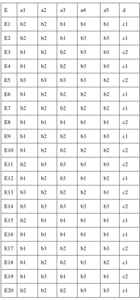
[image:3.595.66.294.251.740.2]To start with we consider initial table which is generated from 20 samples which we get by the method of correlation techniques.
Table-1:
E a1 a2 a3 a4 a5 d
E1 b2 b2 b1 b1 b1 c1
E2 b2 b2 b1 b3 b3 c1
E3 b1 b2 b2 b3 b3 c2
E4 b1 b2 b2 b3 b3 c1
E5 b3 b3 b3 b3 b2 c2
E6 b1 b2 b2 b2 b2 c1
E7 b2 b2 b2 b2 b2 c1
E8 b1 b1 b1 b1 b1 c2
E9 b1 b2 b2 b3 b3 c1
E10 b1 b2 b2 b2 b2 c2
E11 b2 b3 b3 b3 b3 c2
E12 b1 b2 b3 b1 b2 c1
E13 b3 b2 b2 b2 b1 c2
E14 b3 b3 b3 b3 b3 c2
E15 b2 b1 b1 b1 b1 c1
E16 b1 b1 b1 b1 b1 c1
E17 b1 b3 b2 b2 b3 c2
E18 b1 b2 b2 b3 b2 c1
E19 b1 b3 b1 b3 b1 c2
E20 b2 b2 b2 b3 b3 c1
The decision table -1 , takes the initial values before finding the reduct looking at the data table it is found that entities E3,E4, ambiguous in nature so both E3,E4 remove from the relational table -1 to produce the new table as our Table-2
Table -2
E a1 a2 a3 a4 a5 d
E1 b2 b2 b1 b1 b1 c1
E2 b2 b2 b1 b3 b3 c1
E5 b2 b1 b2 b3 b2 c2
E6 b1 b2 b2 b2 b2 c1
E7 b2 b2 b2 b2 b2 c1
E8 b1 b1 b1 b1 b1 c1
E9 b1 b2 b2 b3 b3 c1
E10 b1 b2 b2 b2 b2 c2
E11 b2 b2 b1 b3 b3 c2
E12 b1 b2 b1 b1 b2 c1
E13 b1 b2 b2 b2 b1 c2
E14 b2 b2 b2 b3 b3 c2
E15 b2 b1 b1 b1 b1 c1
E16 b1 b1 b1 b1 b1 c1
E17 b1 b2 b2 b2 b3 c2
E18 b1 b2 b2 b3 b2 c2
E19 b1 b2 b1 b3 b1 c2
E20 b2 b1 b2 b3 b3 c1
4.1 Indiscernibility relation
Indiscernibility Relation is the relation between two or more objects where all the values are identical in relation to a subset of considered attributes.
4.2 Approximation
relation. Below is presented and described the types of approximations that are used in Rough Sets Theory.
4.2.1
Lower Approximation
Lower Approximation is a description of the domain objects that are known with certainty to belong to the subset of interest.The Lower Approximation Set of a set X, with regard to R is the set of all objects, which can be classified with X regarding R, that is denoted as RL
4.2.2
Upper Approximation
Upper Approximation is a description of the objects that possibly belong to the subset of interest. The Upper Approximation Set of a set X regarding R is the set of all of objects which can be possibly classified with X regarding R. Denoted as RU.
Boundary Region is description of the objects that of a set X regarding R is the set of all the objects, which cannot be classified neither as X nor -X regarding R. If the boundary region X= ф then the set is considered "Crisp", that is, exact in relation to R; otherwise, if the boundary region is a set X≠ф the set X "Rough" is considered. In that the boundary region is BR = RU-RL.
The lower and the upper approximations of a set are interior and closure operations in a topology generated by a indiscernibility relation. In discernibility according to decision attributes in this case has divided in to two groups
One groups consist of all positive case and other one all negative cases
E(Success)={ E1, E2, E6, E7, E8, E9 ,E12, E15, E16,E20}…(1)
E(Failure)={ E5, E10, E11, E13, E14 ,E17, E18, }...(2)
Here in this case lower approximation for Success represented by the first equation and lower approximation for failure represented by the Second equation now we find the entities which are falls into different groups to generate different equivalence classes as follows
E(a1)high ={E6, E8, E9, E10, E12, E16 ,E17, E18, E19} E(a1)medium ={E1, E2, E7, E11 ,E15, E20}
E(a1)low =={E5, E13, E14 }, E(a2)high ={E8, E15, E16 }
E(a2)medium ={ E1, E2, E6,E7,E9,E10,E12,E13,E18,E20 } E(a2)low={ E1,E8,E12,E15, E16 }
E(a3)high={ E1,E8,E12,E15, E16 } E(a3)medium={ E6,E7,E10, E13 ,E17 }
E(a3)low={ E5,E11,E12,E14} E(a4)high={ E5,E11,E12,E14 }
E(a4)medium={ E1,E8,E12,E15, E16 } E(a4)low={ E6,E7,E10, E13 ,E17 }
E(a5)high ={E1,E8,E13,E15,E16,E19} E(a5)medium ={E5,E6,E7,E10,E12,E18}
E(a5)low ={E2,E9,E11,E14,E17,E20} Next, we find the combination of two attributes each to generate the reduct such combinations are E(a1,a2), E(a1,a3), E(a1,a4),
E(a1,a5) E(a1,a2)high={E8,E16},
E(a1,a2)medium={E1,E2,E7,E20}
E(a1,a2)low ={E3,E14 } E(a1,a3)high={E8,E16,E19} E(a1,a3)medium ={E7,E20}
E(a1,a3)low ={E5,E14} E(a1,a4)high={E8,E12,E16} E(a1,a4)medium ={E7 } E(a1,a4)low ={E5,E14 } E(a1,a5)high={E8,E12,E16} E(a1,a5)medium ={E7} E(a1,a5)low={E14}
E(a2 , a3)high ={E8,E15,E16} E(a2,,a3)medium ={E6,E7,E9,,E10,E13,E18,E20}, E(a2,,a3)low ={E5,E11,E14} E(a2,,a4)high ={E8,E15,E16}
E(a2,,a4)medium ={E6,E7,E10,E13} E(a2,,a4)low ={E5,E11,E14 } E(a2,,a5)high ={E8,E16 } E(a2,,a5)medium ={E7} E(a2,,a5)low ={E11,E14,E17}
E(a3,,a4)high ={E1,E8,E15,E16} E(a3,,a4)medium ={E6,E7,E1\0,E13,E17}
E(a3,,a4)low ={E5, E11,E14} E(a3,,a5)high ={E1, E8,E15,E16,E19}
E(a3,,a5)medium ={E6, E7,E10,E18 } E(a3,,a5)low ={E11, E14 }
E(a4,,a5)high ={E1, E8 ,E15,E16} E(a4,,a5)medium ={E6, E7 , E10 } E(a4,,a5)low ={E2,E9,E20}
E(a1,a2 ,a3)high={E8,E16} E(a1,a2 ,a3)medium ={E7,E20} E(a1,a2 ,a3)low ={E5,E14}
E(a2,a3 ,a4)high ={E8 ,E15, E16} E(a2,a3 ,a4)medium ={E6 ,E7, E10 ,E13}
E(a2,a3 ,a4)low ={E5 ,E11, E14 } E(a3,a4 ,a5)high ={E1,E8, E15 } E(a3,a4 ,a5)medium ={E6,E7, E10 } E(a3,a4 ,a5)low ={E11,E14}
E(a1,a2,a3,a4)high={E8,E16} E(a1,a2,a3,a4)medium={E7}
E(a1,a2,a3,a4)low={E5,E14} these equivalence classes are basically responsible for finding the dependencies with respect to the decision variable d in this paper besides all equivalence classes , we are trying to find out the degree of dependencies of different attributes of consideration with respect to decision attributes d considering only attribute print media that is E(a1)high/medium(success) or(failure)) cases can’t classified as several ambiguity result found out that is {E2,E5} , {E9,E10}, {E12,E3}, {E14,E15},{E16,E17} with respect to decision variable d so for that print media gives insignificant result so this attribute has hardly any importance. similarly for television advertisement we have to find the degree of dependency (television advertisement attributes rename as a2) E(a2)high/low(success)= {E1,E2,E6,E7,E9,E12, E8, E15,E16,E20} so degree of dependency 10/20 for the success cases with respect to decision variable d similarly the failure cases in television advertisement cases are E(a2)medium (success)={ E8, E15,E16,E20} 4/20 E(a2)medium//high (failure)= { E17, E18,E19} 3/20 for that we can have a significant result for television advertisement that is whether television advertisement is high or medium generally produces positive cases so television advertisement has certain level of significance in business success that is if television advertisement is high that leads to a business success now analyzing localize that is a3 we have the following results E(a3)medium /high(success)= { E1, E2, E6 E7 ,E8,E9 E12,E15,E20} E16,E19 Produces ambiguous result so here the degree dependency 9/20 on success cases two ambiguous cases
similarly the negative cases
E(a3)(negative)medium/high={E10,E11,
like E1, E2, E8,E12 produces the same result that is if localize is moderate then we have success cases similarly analyzing the negative cases we have similar result E5,E6 produces ambiguous result so we are consider these and for other cases E10, E13,E14,E17,E18 produces the same result that is all high localize produces failure result , that if localize is high the still business failure is being observed so upon analyzing the data , advertisement by localize method produces insignificant result that is in some cases this attribute produce success and in some cases it deliver negative result the number in both cases are nearly equal .So for that in case of localize advertisement we can’t generate any definite rule from localize advertisement attribute dropping this attribute from the decision table may hamper the investigation process so we keep this attribute in the decision table for further investigation next we investigate E(a4)medium /high(success) ={ E1,E6, E7,E12,E15,E16} dependency factor for positive cases will be 6/20
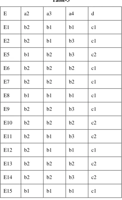
[image:5.595.78.283.431.766.2]E(a4)lowl/medium (failure)={ E5,E11, E14,E18} E19,E20 gives ambiguous result here dependency factor for negative cases will be 4/20 similarly for analyzing indirect advertisement we have E(a5)high /medium (success)={E1,E6, E15} two ambiguity result E8, E13 and E12 ,E18 in failure cases similarly in negative cases E5, E7 are ambiguous result so need not go for further investigation so we can drop two attributes from the tables that is a1,a5 from the table so we are having new table given below . We are considering the definite cases whether failure or success for the cases where we are not sure of the result we keep those attribute in the table for further investigation, the reduct table which we generate presented in Table 3
Table-3
E a2 a3 a4 d
E1 b2 b1 b1 c1
E2 b2 b1 b3 c1
E5 b1 b2 b3 c2
E6 b2 b2 b2 c1
E7 b2 b2 b2 c1
E8 b1 b1 b1 c1
E9 b2 b2 b3 c1
E10 b2 b2 b2 c2
E11 b2 b1 b3 c2
E12 b2 b1 b1 c1
E13 b2 b2 b2 c2
E14 b2 b2 b3 c2
E15 b1 b1 b1 c1
E16 b1 b1 b1 c1
E17 b2 b2 b2 c2
E18 b2 b2 b3 c2
E19 b2 b1 b3 c2
E20 b1 b2 b3 c1
In table 3 we found E1,E12 provides same values similarly E6,E7 also provide the same result and E2,E11 ambiguous result so we keep one table E1 for E1,E12 and keep E6 for E6,E7 and drop both E2,E11 from the tables to leads to table 4
Table 4
E a2 a3 a4 d
E1 b2 b1 b1 c1
E5 b1 b2 b3 c2
E6 b2 b2 b2 c1
E8 b1 b1 b1 c1
E9 b2 b2 b3 c1
E10 b2 b2 b2 c2
E13 b2 b2 b2 c2
E14 b2 b2 b3 c2
E15 b1 b1 b1 c1
E16 b1 b1 b1 c1
E17 b2 b2 b2 c2
E18 b2 b2 b3 c2
E19 b2 b1 b3 c2
E20 b1 b2 b3 c1
From the table -4 we get conclusion that E5,E20 provides ambiguous result so we drop both E5,E20 from the table leads to table table-5
Table-5
E a2 a3 a4 d
E1 b2 b1 b1 c1
E6 b2 b2 b2 c1
E9 b2 b2 b3 c1
E10 b2 b2 b2 c2
E13 b2 b2 b2 c2
E14 b2 b2 b3 c2
E15 b1 b1 b1 c1
E16 b1 b1 b1 c1
E17 b2 b2 b2 c2
E18 b2 b2 b3 c2
E19 b2 b1 b3 c2
Again analyzing table -5 we have E6,E10 produces ambiguous result and { E13,E17 }leads to single results that is E13 so table -5 further reduces to table -6 by deleting the ambiguity and redundancy
Table-6
E a2 a3 a4 d
E1 b2 b1 b1 c1
E8 b1 b1 b1 c1
E9 b2 b2 b3 c1
E13 b2 b2 b2 c2
E14 b2 b2 b3 c2
E15 b1 b1 b1 c1
E16 b1 b1 b1 c1
E18 b2 b2 b3 c2
E19 b2 b1 b3 c2
Now further classification E15,E16 leads to same class that is{ E15,E16 }= E15 further reduction produces table-7 by deleting the redundant rows.
Table-7
E a2 a3 a4 d
E1 b2 b1 b1 c1
E8 b1 b1 b1 c1
E9 b2 b2 b3 c1
E13 b2 b2 b2 c2
E14 b2 b2 b3 c2
E15 b1 b1 b1 c1
E18 b2 b2 b3 c2
E19 b2 b1 b3 c2
Continuing the reduction process we further reduces E14,E18 giving the same conclusion both leads to same result which generate the reduction table as table-8
Table-8
E a2 a3 a4 d
E1 b2 b1 b1 c1
E8 b1 b1 b1 c1
E9 b2 b2 b3 c1
E13 b2 b2 b2 c2
E14 b2 b2 b3 c2
E15 b1 b1 b1 c1
E19 b2 b1 b3 c2
The same procedure again gives us further reduction that is E8, E15 also leads to same information sets so futher reduction gives another tale named as table-9
Table-9
E a2 a3 a4 d
E1 b2 b1 b1 c1
E8 b1 b1 b1 c1
E9 b2 b2 b3 c1
E13 b2 b2 b2 c2
E14 b2 b2 b3 c2
E19 b2 b1 b3 c2
Here in table -9 again we have E9,E14 leads to ambiguous results so dropping both the table for further classification we have table-10
Table-10
E a2 a3 a4 d
E1 b2 b1 b1 c1
E9 b2 b2 b3 c1
E13 b2 b2 b2 c2
E19 b2 b1 b3 c2
Now next we find the the strength[27] of rules for attributes a2, a3, a4 strength of rules for attributes define as strength for an association rule x→D define as is the the number of examples that contain xUD to the number examples that contains x
(a2=b2)→(d=c1)=2/3=66%
,(a2=b1)→(d=c1)=1=100%,,(a2=b2)→(d=c2)=2/4=25%, (a2=b1)→(d=c2)=nil now we calculate strength for a3 (a3=b1)→(d=c1)=2/3=66%,(a3=b2)→(d=c1)=1/2=50%,(a3 =b1)→(d=c2)=1/3=33%,
(a3=b2)→(d=c2)=1/2=50
Similarly strength for a4 will be (a4=b1)→(d=c1)=1 =100% (a4=b2)→(d=c1)=1=100%,(a4=b1)→(d=c2)=nil (a4=b3)→(d=c2)=1/2=50%, (a4=b2)→(d=c2)=100%
In this analysis we find a2 and a3 must important attributes in analyzing the data analysis as because we are having a result for a4 that is high marketing gives a failure result so the conditional attribute a4 is not that important like a2,a3 from the above analysis we develop a rule that is
1.(a2)medium /high→ shows a success that is a2 is medium or high leads to business success similarly
For (a3 ) medium/high→ may leads to a business success but still there is a 50% chances of failure also exit in high localize cases
4.3 Statistical validation
We basically focus on sample size for our paper , we consider a sample size of 1000 , although we get a conclusion . As rough set deals with uncertainty may leads to some kind of confusion regarding the result to validate our claims we depends upon chi squared test to validate our claim by using chi squared test
We found that chi squared value that is chi squared value we consider as k which lies below the critical range
4.4 Experimental section
We take survey of different successful business organization adopting the rule generated by rough set principle are as follows
Expected15%,10%,15%,20%,30%,15% and the Observed samples are 25,14,34 45,62,20 so totaling these we have total of 200 samples so expected numbers of samples per each day as follows 30,20,30,40,60,30 . We then apply chi square distribution to verify our result assuming that H0 is our hypothesis that is correct H1 as alternate hypothesis that is not correct , Then we expect sample in six cases as
chi squared estimation formula is ∑(Oi-Ei)2/ Ei where i=0,1,2,3,4,5 so the calculated as follows X2=(25- 30)2/20+(14-20)2/20+(34-30)2/30+(45-40)2/40+(62-60)2/60+(20-30)2/30
X2=25/20+36/20+16/30+25/40+4/60+100/30
=7.60 the tabular values we have with degree of freedom 5 we get result 11.04
Our experiment result is lies quite below the tabular values, so it lies in the acceptable region .So we accept the hypothesis H0 that of our experiment result is correct.
5.FUTURE WORK
Our work can be extended to different fields like student feedback system, Business data analysis, Medical data analysis
6.CONCLUSION
This is based upon mathematical analysis and experiment which is gives some accurate result in generating rules, from a vast diversified data base. This also gives a very précised result
7.REFERENCES
[1] S.K. Pal, A. Skowron, Rough Fuzzy Hybridization: A new trend in decision making, Berlin, Springer-Verlag, 1999
[2] Z. Pawlak, “Rough sets”, International Journal of Computer and Computer and Information Sciences, Vol. 11, 1982, pp.341–356
[3] Z. Pawlak, Rough Sets: Theoretical Aspects of Reasoning about Data, System Theory, Knowledge Engineering and Problem Solving, Vol. 9, The Netherlands, Kluwer - Academic Publishers, Dordrecht, 1991
[4] Han, Jiawei, Kamber, Micheline, Data Mining: Concepts and Techniques. San Franciso CA, USA, Morgan Kaufmann Publishers, 2001
[5] Ramakrishnan, Naren and Grama, Y. Ananth, “Data Mining: From Serendipity to Science”, IEEE Computer, 1999, pp. 34-37.
[6] Williams, J. Graham, Simoff, J. Simeon, Data Mining Theory, Methodology, Techniques, and Applications (Lecture Notes in Computer Science/ Lecture Notes in Artificial Intelligence), Springer, 2006.
[7] D.J. Hand, H. Mannila, P. Smyth, Principles of Data Mining. Cambridge, MA: MIT Press, 2001
[8] D.J. Hand, G.Blunt, M.G. Kelly, N.M.Adams, “Data mining for fun and profit”, Statistical Science, Vol.15, 2000, pp.111-131.
[9] C. Glymour, D. Madigan, D. Pregibon, P.Smyth, “Statistical inference and data mining”, Communications of the ACM, Vol. 39, No.11,1996, pp.35-41.
[10]T.Hastie, R.Tibshirani, J.H. Friedman, Elements of statistical learning: data mining, inference and prediction, New York: Springer Verlag, 2001
[11]H.Lee, H. Ong, “Visualization support for data Mining”, IEEE Expert, Vol. 11, No. 5, 1996, pp.
69-75.
[13]E.I Altman, “Financial ratios, discriminants analysis and prediction of corporate bankruptcy”, The journal of finance, Vol. 23 , 1968, pp.589-609
[14]E.I.Altman, R.Avery, R.Eisenbeis, J. Stnkey, “Application of classification techniques in business, banking and finance. Contemporary studies in Economic and Financial Analysis”, vol.3, Greenwich, JAI Press,1981.
[15]E.I Altman, “The success of business failure prediction models: An international surveys”, Journal of Banking and Finance Vol. 8, no.2, 1984, pp.171-198
[16]E.I Altman, G. Marco, F. Varetto, “Corporate distress diagnosis: Comparison using discriminant analysis and neural networks”, Journal of Banking and Finance, Vol. 18, 1994, pp. 505-529
[17]W.H Beaver, “Financial ratios as predictors of failure. Empirical Research in accounting : Selected studies”, Journal of Accounting Research Supplement to Vol 4, 1966, pp.71-111
[18]J.K Courtis, “Modelling a financial ratios categoric frame Work”, Journal of Business Finance and Accounting, Vol. 5, No.4, 1978, pp71-111
[19]H.Frydman, E.I Altman ,D-lKao, “Introducing recursive partitioning for financial classification: the case of financial distress”, The Journal of Finance, Vol.40, No. 1, 1985, pp. 269-291.
[20]Y.P.Gupta, R.P.Rao, P.K. , Linear Goal programming as an alternative to multivariate discriminant analysis a note journal of business fiancé and accounting Vol.17, No.4, 1990, pp. 593-598
[21]M. Louma, E, K. Laitinen, “Survival analysis as a tool for company failure prediction”. Omega, Vol.19, No.6, 1991, pp. 673-678
[22]W.F. Messier, J.V. Hanseen, “Including rules for expert system development: an example using default and bankruptcy data”, Management Science, Vol. 34, No.12, 1988, pp.1403-1415
[23]E.M. Vermeulen, J. Spronk, N. Van der Wijst., The application of Multifactor Model in the analysis of corporate failure. In: Zopounidis,C.(Ed), Operational corporate Tools in the Management of financial Risks, Kluwer Academic Publishers, Dordrecht, 1998, pp. 59-73
[24]C. Zopounidis, A.I. Dimitras, L. Le Rudulier, A multicriteria approach for the analysis and prediction of business failure in Greece. Cahier du LAMSADE, No. 132, Universite de Paris Dauphine, 1995.
[25]C. Zopounidis, N.F. Matsatsinis, M. Doumpos, “Developing a multicriteria knowledge-based decision support system for the assessment of corporate performance and viability: The FINEVA system, “Fuzzy Economic Review, Vol. 1, No. 2, 1996, pp. 35-53.
[26]C. Zopounidis, M. Doumpos, N.F. Matsatsinis, “Application of the FINEVA multicriteria knowledge- decision support systems to the assessment of corporate failure risk”, Foundations of Computing and Decision Sciences, Vol. 21, No. 4, 1996, pp. 233-251
![arxiv: v4 [physics.plasm-ph] 21 Jun 2016](data:image/gif;base64,R0lGODlhAQABAIAAAP///wAAACH5BAEAAAAALAAAAAABAAEAAAICRAEAOw==)