Munich Personal RePEc Archive
Flood Insurance Coverage in the Coastal
Zone
Landry, Craig E. and Jahan-Parvar, Mohammad R.
East Carolina University
November 2008
Online at
https://mpra.ub.uni-muenchen.de/15498/
Flood Insurance Coverage in the Coastal Zone
Craig E. Landry*
Associate Professor, Department of Economics Assistant Director, Center for Natural Hazards Research
East Carolina University 252-328-6383 (p); 252-328-6743 (f)
and
Mohammad R. Jahan-Parvar
Assistant Professor, Department of Economics East Carolina University
252-328-4770 (p); 252-328-6743 (f) [email protected]
Department of Economics working paper ecu0804
November 2008
* Craig Landry is author for correspondence. Thanks to Robert Hoyt, Andrew Keeler, Warren Kriesel, and
seminar participants at the University of Georgia for their input, and to the H.J. Heinz III Center for Science, Economics, and the Environment and the Federal Emergency Management Agency for their roles in supporting and assisting in data collection. We thank Haiyong Liu for his comments. This research was partially supported by a North Carolina research competitiveness grant. Craig Landry gratefully
Flood Insurance Coverage in the Coastal Zone
Abstract
We explore behavior and test theory regarding the determinants of flood insurance coverage in the coastal zone using household-level data for nine southeastern counties. We use Tobit regression models to assess the importance and magnitude of insurance cost, risk factors, community characteristics, and household attributes on flood insurance purchase for residential building structures. Overall estimates indicate price inelastic demand, though subsidized policyholders are more sensitive to price and hold greater flood insurance coverage (controlling for value of asset at risk). We find support for rational choice in the coastal zone, with flood insurance coverage positively correlated in the level of flood risk. We find evidence that coastal erosion risk effects flood insurance demand, and that community level erosion hazard mitigation projects influence flood insurance holdings, with shoreline armoring appearing to act as a substitute and beach replenishment appearing to act as a complement.
Key words: Insurance coverage, flood, hazard, coastal, erosion, Tobit model
Flood Insurance Coverage in the Coastal Zone
Introduction
Over the past 50 years, coastal areas in the United States have witnessed a growing
populace, an evolving social environment, and increased economic activity. On the East
and Gulf coasts, the burgeoning population faces considerable risk from coastal storms
(hurricanes and nor’easters) that periodically cause extensive flooding, wind, and erosion
damage. Increasing coastal populations, development in hazard-prone areas, rising
construction costs and increased value at risk have contributed to rising monetary losses
due to these natural hazards (Kunreuther 1998a; Wharton 2008). Nordhaus (2006)
estimates the value of capital stock in low-lying coastal areas vulnerable to natural
hazards at $1.2 trillion (about 3% of GDP (2005 dollars)), and recent predictions suggest
that we are entering a period of increased storm activity (Goldenberg et al. 2001; Webster
et al. 2005) which could exacerbate coastal risk.
Historically, the catastrophic nature of flood risk and government’s predilection
for disaster aid has precluded private insurers from voluntarily offering coverage
(Anderson 1974, Kunreuther 1998b). Since the late 1960s, the U.S. federal government
has played an expanded role in providing protection from flood and other coastal hazards.
The National Flood Insurance Act of 1968 made federal flood insurance available,1
through the National Flood Insurance Program (NFIP), to communities that agreed to
manage development in floodplains, with subsequent legislation (Flood Disaster
Protection Act of 1973, National Flood Insurance Reform Act of 1994) designed to
1
augment incentives for insurance purchase and hazard mitigation projects (Pasterick
1998). The National Flood Insurance Reform Act of 1994 charged the Federal
Emergency Management Agency (FEMA) with evaluating the effects of coastal erosion
on coastal communities and the NFIP (Heinz Center 2000). In light of increasing coastal
populations and predictions of increasing coastal storm intensity, there is heightened
concern about natural hazard exposure in coastal areas and the viability of NFIP.
Understanding household demand for coverage is a key element in assessing the viability
of the market for flood insurance and the role of market insurance vis-à-vis and in
conjunction with other forms of indemnification from coastal hazards.
Due to the large number and diversity of affected communities, delineation of
flood risk under the Flood Disaster Protection Act of 1973 proved a laborious task,
leading to the development of the NFIP in phases. The “Emergency Phase” of the
program offered insurance at subsidized rates to households in communities that agreed
to adopt floodplain management ordinances. Subsidized insurance rates applied only
until detailed Flood Insurance Rate Maps (FIRMs) could be produced, after which new
construction would pay “actuarial” rates determined by location in the flood zone,
structural characteristics (e.g., elevation), and the existence of community hazard
mitigation projects (in the “Regular Phase” of the program).2 Construction after the
publication of FIRMs was required to meet new building standards designed to make
structures more flood resistant. As of 1997, 35% of properties in the flood zone
2
nationwide were eligible for explicitly subsidized insurance, paying approximately 37%
of the actuarial premium (Burby 2001).3
Since its inception, the NFIP has suffered from low levels of participation among
homeowners. The Flood Disaster Protection Act of 1973 required communities be
enrolled in NFIP in order to qualify for certain types of federal disaster assistance and
required flood insurance purchase for federally-backed (FHA) mortgage loans in
high-risk areas (Pasterick 1998). Mandatory purchase requirements were strengthened under
the National Flood Insurance Reform Act of 1994, and programs were expanded to
encourage local hazard mitigation projects. Nonetheless, evidence suggests that
mandatory purchase requirements are not aggressively enforced after the initial year of a
mortgage contract (Kunreuther 1996; Palm 1998; Tobin and Calfee 2005), so that after a
loan is secured participation becomes de facto voluntary.4 In 1997, market penetration
for the NFIP across the U.S. was estimated at 26% of eligible parcels
(PricewaterhouseCoopers 1999). Explanations for low market penetration have included
ignorance of and lack of experience with flood hazard, subjective misperceptions of the
likelihood of flooding and magnitude of loss, lack of awareness of the availability of
flood insurance or belief that the price is too high, and “charity hazard” ― a reliance on
assistance from others (e.g. government) in the event of disaster (Kunreuther 1984, Lewis
and Nickerson 1989, Kunreuther 1996, Browne and Hoyt 2000).
In this paper, we focus on flood insurance coverage choice in the coastal zone,
utilizing household micro-data from 6074 parcels in nine southeastern U.S. counties.
3
The Congressional Budget Office estimates that the extent of subsidy has dropped to 25% of policies as of 2005 (Marron 2006).
4
These data were collected by the H.J. Heinz III Center for Science, Economics, and
Environment, under the direction of FEMA, pursuant to addressing questions regarding
the impact of shoreline erosion on coastal communities and the NFIP (Heinz 2000), and
were utilized by Kriesel and Landry (2004) to examine participation in the NFIP. We
expand upon their analysis in a number of ways: i) our empirical model considers not
only participation, but also the level of coverage elected; ii) we improve upon the
insurance premium covariate by employing NFIP rate schedules to determine marginal
price measures that reflect specific property risk attributes (rather than average imputed
prices as employed in Kriesel and Landry (2004)); and iii) we explore a greater array of
specifications and covariates in our analysis in order to test economic and behavioral
determinants of flood insurance coverage.
Consistent with previous research, we find evidence of price inelastic demand for
flood insurance. Price elasticity varies across subsidized and non-subsidized insurance
policies, with subsidized policyholders exhibiting greater overall coverage (controlling
for the value of asset at risk) and elastic demand. Our findings provide support for
rational choice theory in general, with coverage demand greater in the highest risk
(V-zone) areas and lower in the least risk (B/C/X-(V-zone) areas relative to more moderate risk
(A-zone) areas (controlling for insurance price and value at risk).
Coverage is increasing in the erosion rate at the nearest shoreline and higher for
those households that claim to possess knowledge of the erosion rate at the nearest shoe,
suggesting that erosion risk may induce flood insurance purchase.5 Further, we find
evidence that coverage is higher in areas that manage erosion through beach
5
replenishment and lower in areas that are structurally fortified, suggesting a difference
between the way households view community protection policies vis-à-vis formal
insurance (complementary in the case of beach replenishment and as a substitute in the
case of shoreline armoring). Results of the extended models suggest that flood insurance
is a normal good, and demand is increasing in the level of education.
Flood Insurance Coverage: Theory and Empirics
Optimal insurance coverage has been analyzed within an expected utility (EU)
maximization framework by Smith (1968) and Mossin (1968). We briefly sketch a
simple version of the model in the context of flood insurance. Let utility U(•) be defined
over individual wealth, Y = A + L, with A representing endowed wealth and L the value
of property exposed to risk. Assume risk aversion: U′(Y) > 0 and U″(Y) < 0. The
probability of loss L is π. The individual may purchase insurance coverage C, providing
indemnity under the loss scenario, with 0 ≤ C ≤ L. The insurance premium is
proportional to C, given by pC. The individual purchase decision problem is:
) (
) 1 ( ) ) 1 ( ( )] ( [
max EU Y U A p C U A L pC
C = =π + − + −π + − , (1)
where C is the object of optimization. It is widely recognized that maximization of (1)
implies full coverage (C = L) if insurance is actuarially fair (p = π) and less than full
coverage is if the premium includes a loading factor (p = (1+λ)π for 0 < λ < 1).6
Introducing an exogenous constant deductible to the loss state increases optimal
coverage, while a piecewise linear pricing schedule will not alter the nature of the
solution as long as unit price on initial coverage (p1) is less than the unit price of
6
subsequent coverage (p2); this is the premium structure for the NFIP, with p1 applying to
initial structure coverage ($0 - $50,000), and p2 applying to additional coverage ($50,000
- $250,000 [the upper limit on structure coverage]).7
Camerer and Kunreuther (1989) observe that public perceptions of risk often
differ from expert objective assessments. Optimal insurance coverage changes in
predictable ways if one allows for subjective loss probabilities across individuals that
differ from objective assessments of insurers; downward bias in subjective risk
assessment reduces optimal coverage, ceteris paribus, as the insurance will appear too
expensive. A number of plausible decision making heuristics give rise to what are
considered behavioral anomalies in the context of EU and lead to systematic errors in
optimization; behavioral anomalies include optimism bias (i.e. “it can’t happen to me”),
desire to reduce anxiety about risk, concerns about the appearance of prudence when
others learn about one’s decisions, wanting to behave as others (i.e. influence of social
norms), and a tendency to ignore low probability events (Camerer and Kunreuther 1989;
McClelland, Schulze, and Coursey 1993; Kunreuther 1996; Palm 1998; Krantz and
Kunreuther 2007). Lack of information on probabilities and magnitudes of loss may
invalidate the EU framework in (1), while saliency of accurate risk information may vary
over time and by context (Kunreuther, Sanderson, and Vetschera 1985; Krantz and
Kunreuther 2007). On the other hand, if full insurance is legally required with strictly
enforced provisions, insurance coverage may not be an object of discretionary choice.
Variations in optimal coverage choice can also be explored through the introduction of
different forms of utility in (1) (e.g. Braun and Muermann 2004; Lee 2007). Though not
7
As long as p1 < p2, the kinked budget constraint still produces a convex set of consumption possibilities
explicitly considered in model (1), the likelihood and expected magnitude of disaster
assistance may affect the demand for flood insurance.
There exists little empirical work on flood insurance coverage. Baumann and
Sims (1978) find evidence that past experience with disasters motivates insurance
adoption, as do social class and personality.8 Survey research suggests that lower income
and non-white households, women, and elderly all tend to exhibit greater fear of
disasters, though it is unclear whether this fear translates into insurance purchase or other
types of mitigation and protective behavior (Palm 1998). Brown and Hoyt (2000) use
state level panel data to estimate a flood insurance demand model. They find a negative
price effect (inelastic in a market penetration model and approximately unitary in a
coverage level model) and positive income effect on flood insurance demand. Consistent
with previous findings, their results suggest that demand is increasing in flood damages
of the prior year. Contrary to expectations, they find that insurance demand is decreasing
in the number of federally-backed (FHA) mortgages and increasing in the amount of
federal disaster assistance.
National data gathered by Dixon et al. (2006) support the finding that market
penetration rates are not sensitive to price, and further suggest that penetration is
significantly higher in special flood hazard areas (SFHA — also known as A-zone)9 and
higher for communities with a larger number of parcels in the SFHA. The authors
attribute the latter finding to more aggressive marketing of and more familiarity with
flood insurance on the part of insurers in such communities. Dixon et al. (2006) find that
8
Baumann and Sims find that the internal-external locus of control is significantly related to insurance adoption, with those who feel that they are in control of their destinies are more likely to hold insurance than those he feel their lives to be directed by external forces.
9
the probability of purchasing insurance is substantially higher in communities subject to
coastal flooding than in communities that are not―63 percent versus 35 percent. They
speculate that demand for flood insurance may be lower in communities not subject to
coastal flooding because there is less appreciation for flood risk or because the type of
coverage offered by flood insurance policies is less attractive in inland areas.
Michel-Kerjan and Kousky (2008) examine county-level panel data and
individual-level policy data to explore characteristics of the flood insurance market in
Florida (which represents approximately 40% of policies in force and total dollars of
coverage). They find that the overwhelming majority of policyholders elect the lowest
level of deductible ($500), and that coverage levels have increased in reaction to the
floods of 2004, while deductibles have decreased. For most policyholders, the $250,000
limit on structure coverage is not binding, as their replacement value is less than this
limit. Further, they find that Florida’s average flood insurance premium is the lowest in
the nation, and surprisingly, the average Florida premium level has decreased in the most
recent year of their data.
Kriesel and Landry (2004) use household level data from the coastal zone to
examine participation in NFIP. They find price inelastic demand for flood insurance and
a positive income effect. Consistent with NFIP requirements their results suggest that
mortgaged properties are much more likely to be covered by flood insurance. Further
they find that insurance participation is higher in coastal areas that are fortified with
artificial erosion protection (shoreline armoring and/or beach replenishment), lower for
properties located further back from the shoreline, and lower for geographical areas that
We expand upon the analysis of Kriesel and Landry by considering both
participation and coverage level in our empirical model, employing different measures of
flood insurance premiums, and explore a greater array of specifications and covariates in
our analysis in order to test economic and behavioral determinants of flood insurance
coverage. Our approach is more similar to the analysis of Guiso and Jappelli (1998),
which examines casualty insurance in Italy and how coverage is influenced by
uninsurable household wealth risk and other factors.
Flood Insurance Coverage Data
We make use of flood insurance coverage data studied by Kriesel and Landry (2004), but
append a complement of information in order to conduct additional analysis. These data
were gathered by the H.J. Heinz III Center for Science, Economics, and the Environment,
under the direction of FEMA, to address issues of flood insurance and coastal erosion.
The sampling frame is residential parcels in the near-shore zone10 of nine coastal counties
in Delaware, North Carolina, South Carolina, Georgia, Florida, and Texas. A stratified
random sample of the near-shore zone was selected across the nine counties using a
T-shaped sampling frame within each county in order to ensure adequate coverage on the
oceanfront; weights are used to adjust all reported statistics for representation of the
near-shore zone.
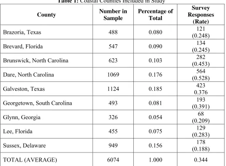
Table 1 displays a breakdown of the 6074 parcels that were selected for the study.
Galveston County, Texas and Dare County, North Carolina provide the most
observations (18.5% and 17.6% of the sample, respectively), while Lee County, Florida
10
and Glynn County, Georgia provide the fewest (7.5% and 5.4% of the sample,
respectively). For each parcel, contractors made onsite visits to collect information, such
as structure elevation above base flood elevation (BFE), foundation type, presence of
basement or other obstruction below the main floor, ocean frontage, etc. Geographic
information systems were employed to estimate distance from the shoreline, distance
from the central business district, flood zone, and historical erosion rate. Parcel and
structure characteristics from the county tax assessor’s database were appended to the
onsite data.11 The sample was then merged by address with the Federal Insurance
Administration’s policies-in-force database in order to provide accurate information on
market penetration and coverage levels. Of the 6074 parcels with complete data, 52
percent of property owners were identified as holders of flood insurance. Lastly, the
dataset was complemented with information from a survey questionnaire sent to the home
address of all parcel owners in the sample during 1998. The response rates, indicated in
the last column of table 1, vary significantly across counties, with a high of 53% in Dare
County, North Carolina and a low of 19% in Sussex County, Delaware. The overall
survey response rate was 34%.
Table 2 reports weighted descriptive statistics on insurance, parcel, and structure
characteristics for the entire sample. The average flood insurance coverage for structure
in the sample (obtained from both policies-in-force data and mail survey) was $71,600
($1998), with a minimum of zero and a maximum of $250,000.12 Average coverage for
NFIP participants was $142,431. The next two rows of table 2 indicate measures of
marginal flood insurance premium expressed in dollars per $100 coverage. Marginal
11
Details of the data collection effort are available in Heinz Center (2000).
12
premiums were calculated using descriptive information on the property and detailed
NFIP rate tables from 2004 (adjusted back to 1998 levels).13 At the parcel level, flood
insurance premiums depend upon a number of factors, including: flood zone, year of
construction relative to publication of FIRM, presence of basement or obstruction below
a property, type of structure, elevation above BFE, Community Ratings System (CRS)
score, the level of coverage, and chosen deductible.14 We discuss each of these factors in
turn.
Most of the properties in our data (50%) are located in the V flood zone, 100-year
flood zone with additional risk due to high-velocity waves associated with storm surge.
Forty-one percent are located in the standard SFHA or A-zone (100-year flood zone), and
9% are located in the B/C/X-zones (500-year flood or lower risk zones). Houses built
before the publication of FIRMs in their community and those in the V-zone built
between 1975 and 198115 are “grandfathered” in the NFIP and pay explicitly subsidized
insurance rates. Fifty-seven percent of the parcels in our dataset qualified for subsidized
insurance under these guidelines. Subsidized and regular flood insurance premiums vary
by flood zone, with structures in the V-zone paying the highest rates and structures in the
X-zone paying the lowest rates. Subsidized rates vary according to whether a basement
or other obstruction is present and by type of structure (single or multiple-family).
Regular rates vary by number of building stories, presence of basement or obstruction,
structure type, and elevation above BFE. Post-FIRM structures with greater elevation
13
Flood insurance rates have been generally increasing over time. Between 1998 and 2004 there were three targeted rate increases that we had to factor into our marginal premium calculations.
14 Total premium also includes a $30 Federal Policy Fee that applies to high-risk areas, an Increased Cost
of Compliance coverage premium, and a Probation Surcharge (if applicable). These additional fees do not affect the marginal premium, but may induce price differences on the extensive margin.
15
pay lower rates. Almost 70% of structures in our dataset are elevated on piles, and 18%
have obstructions below the property. Average elevation above base flood elevation
(BFE height of the 100year flood) was 3.3 feet, with a high of 30 feet and a low of
-12.5 feet (that is -12.5 feet below BFE).
The National Flood Insurance Reform Act of 1994 established the Community
Rating System (CRS) to evaluate and summarize mitigation projects in a community.
The CRS score ranges from 1 (many mitigation projects, low flood risk) to 10 (little or no
mitigation projects, baseline flood risk); a lower CRS score decreases flood insurance
premiums. The average CRS score for our sample was 8.3 with a low of 5 and a high of
10. All premiums are adjusted to reflect the CRS score for the community, with
discounts ranging from 0% (for a score of 10) to 25% (for a score of 5).
Premiums also vary by amount of coverage. A basic lower rate applies to the first
$50,000 of coverage on structure, while a higher rate applies to additional coverage up to
the $250,000 limit on structure.16 Knowing coverage level, we are able to apply the
marginal rate in our empirical analysis. The marginal rate should affect decision making
via the theoretical model in (1). Previous research (Kriesel and Landry 2004) has
employed an estimate of the average insurance rate.
The standard deductible for NFIP structure coverage is $500. Reduced premiums
are awarded for those opting for a higher deductible, up to $5,000 deductible on
single-family structures. Premiums for post-FIRM structures in the V-zone built after 1981
(approximately 14% of our data) depend upon the ratio of coverage level to replacement
value (‘replacement cost ratio’). Unfortunately, our data contain limited information (N
16
= 1668 for policy holders) on deductible level17 and no information on replacement
value.18 To make full use of the available data, we consider two measures of marginal
premium ― a high and a low version ― in order to assess the responsiveness of coverage
demand to premium level. The high premium model assumes all households elect the
standard $500 deductible and that post-FIRM structures in the V-zone built after 1981
select a level of coverage that is less than 50% of the structure replacement cost. The
data of Michel-Kerjan and Kousky (2008) suggest that 98% of Florida policyholders
select a deductible less than the maximum and 80% choose the lowest deductible of
$500. Thus, the high premium assumptions probably provide the most accurate results.
The average high marginal premium is $1.01 per $100 coverage with a minimum of
$0.06 and a maximum of $6.00. The price elasticity from the coverage model that
employs the high marginal premium will be a lower bound on the true value. The low
premium model assumes all households elect a $1000 deductible and that post-FIRM
structures in the V-zone built after 1981 select a level of coverage that is greater than or
equal to 75% of the replacement cost. The average low marginal premium is $0.87 per
$100 coverage with a minimum of $0.06 and a maximum of $3.90. The price elasticity
from the coverage model that employs the low marginal premium will be an upper bound
on the true value.
The average historical beach erosion rate is 2.7 feet per year for those properties
in an actively eroding zone (71% of the sample). A much smaller proportion (6.5%) or
parcels are in accreting zones, with an average accretion rate of 0.2 feet per year. The
remaining 22.5% of parcels are classified as being in neither an erosion or accretion
17
Of these data, 50% claim structure deductible of $500 and 80% claim deductible of $1000 or less.
18
zone.19 Kriesel, Randall and Lichtkoppler (1993) use a variable transformation, geotime,
to measure erosive pressure on a parcel. Geotime is defined as the ratio of setback (or
distance from the shoreline) to historical erosion rate, providing an estimate of the
number of years a parcel is expected to remain in the face of constant, deterministic
shoreline erosion. Average geotime in our sample is 787 years, but approximately 30%
of the parcels exhibited geotime less than 10 years. The hurricane return period, the
mean number of years expected to elapse between landfall of major hurricanes in an area,
was calculated at the county level from summary information provided by FEMA. The
average is 47 years, with a low of 16 years and a high of 190 years. The average distance
from the shore is 318 feet and 42% of properties are oceanfront.
The tax assessor’s database provides information on assessed building and land
values, recent sales price, year of construction, year of sale, and other structural variables.
Building and land assessed values are unreliable measures of value for our analysis due to
differences in assessment and updating across municipalities. Since information on sales
price is limited (N = 2844), we employ hedonic price regression to produce imputed
current property values.20 The average property sales price is $187,177 (1997$), and the
average predicted asset value is $143,683. The average ratio of flood insurance coverage
to estimated asset value is 0.651. Year of construction is used to determine whether the
structure was built after the publication of a FIRM in the community. Post-FIRM
buildings are required to meet more stringent building standards and pay ‘actuarial’ flood
insurance rates.
19
The erosion rates were calculated by state coastal zone managers. In some cases, managers set the erosion rate to zero if structural fortification (i.e. seawalls) were in place.
20
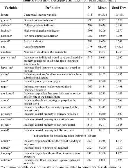
We turn next to survey data gathered from the mail questionnaire. The
descriptive statistics are weighted for non-response bias of NFIP non-participants (in
addition to the T-shaped sampling frame) and are presented in table 3. Household
income is measured by a nominal response to 8 income categories, with the mid-point
utilized as an estimate. The average income is over $100,000. Twenty percent of
respondents have high school as the highest level of educational attainment; 43% are
college graduates, and 36% have at least some graduate school training. Forty-five
percent are retired, and 5% work part-time. The average age is 61 years, and the average
household has 0.46 children.
Sixty-eight percent of respondents indicated that they would have purchased their
coastal home regardless of whether flood insurance was available, and 11% indicate that
they have allowed their flood insurance to lapse at some time in the past. Ten percent
indicate that they have submitted an insurance claim for flood damages in the past.
Thirty-nine percent identify their property as mortgaged, but surprising only 15% claim
that they were required to purchase flood insurance by their mortgage lender. Only 28%
of respondents claimed to be aware of the erosion rate at the nearest shore. Nineteen
percent indicated that shoreline armoring was being used to combat erosion at the
shoreline nearest their property, while 35% indicated that beach replenishment was being
utilized at the nearest shoreline. The majority of respondents (35%) utilize their property
as a vacation home. Thirty percent use the property as part-time rental and part-time
vacation home. Almost a quarter utilize the property as their primary residence, and 10%
A subset of respondents (N = 292) provided information regarding why they did
not hold flood insurance. The majority (30%) indicated that flood insurance was too
expensive. A quarter indicated that they perceived the risk of flooding as very low, while
20% claimed they were not required to purchase flood insurance. Nine percent indicated
that flood insurance was unavailable.
Econometric Models of Flood Insurance Coverage
We employ multiple regression analysis to explore determinants of flood insurance
coverage choice for residential building structures in the near-shore coastal zone. We
consider two models, one of coverage level with imputed asset value included as a
covariate (referred to as the ‘coverage’ model), and the other of the ratio of coverage
level to imputed asset value (referred to as the ‘ratio’ model). Flood insurance coverage
is a censored variable because it cannot be below $0 (and for the coverage model, it
cannot exceed the $250,000 upper limit). We use the Tobit model (Tobin 1958,
Wooldridge 2001), which assumes that the continuous portion of the error distribution is
reasonably approximated by a Gaussian probability density, while the censored values are
represented by cumulative Gaussian probability masses. Due to the use of an imputed
regressor in the coverage model, we use bootstrapping to obtain reliable standard errors.
Let yi be the amount of flood insurance coverage elected, or the ratio of coverage
to asset value. The dependent variable for a Tobit model can be censored as follows:
⎪ ⎩ ⎪ ⎨ ⎧ < ≤ ≤ > = LL y LL UL y LL y UL y UL y i i i i i * * * * ; ; ;
where yi is the observed response variable (coverage level or ratio of coverage to asset
value), is the latent response variable, UL is the upper limit on coverage ($250,000)
and LL is the lower limit ($0). The upper limit applies only to the coverage model. The
log-likelihood function for the Tobit model is: * i y ) ' ( ln ) ' ( 1 ln ) ' ( ln } { } { }
{
∑
= ∈∑
< < ∈∑
=∈ − − Φ + − + − Φ = UL y i i UL y LL i i i LL y i i i i i x UL x y x LL LF σ β σ β φ σ σ β (3)
for the coverage model, and:
) ' ( 1 ln ) ' ( ln } { }
{
∑
= ∈∑
< < ∈ − + − Φ = UL y LL i i i LL y i i i i x y x LL LF σ β φ σ σβ (3’)
for the ratio model, where φ(•) represents the standard normal probability density
function, represents the standard normal cumulative distribution function, x is a
vector of covariates hypothesized to effect demand for flood insurance coverage, and β
and σ parameters to be estimated. )
(•
Φ
Economic theory provides guidance on the specification of covariates for our
regression models (Smith 1969, Mossin 1969). The marginal price of flood insurance
(i.e. the amount charged for additional $100 coverage) is a primary parameter in the
specification of demand, as is household income. Risk factors, such as presence in a
flood zone, should affect demand; we hypothesize that households in higher risk zones
will demand greater coverage, but the higher cost of insurance in these zones makes the
effect uncertain. We also explore erosion hazard factors, such as the erosion/accretion
rate and the presence of erosion mitigation projects (shoreline armoring or beach
replenishment) in the nearby area. Households may view such projects as substitutes or
protection offered. Other covariates in the model include property usage and household
demographic factors.
Theory and intuition suggest that the value of the asset at risk should affect
insurance demand. Unfortunately, we have limited information on property replacement
values. We employ hedonic price regression analysis to produce imputed current
property values, and take a proportion of the imputed value as an estimate of the
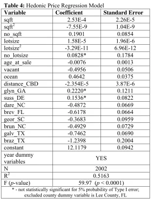
replacement value of the structure at risk. The hedonic price regression parameters for
the entire sample are displayed in table 4. The estimation utilizes a semi-log functional
form and includes housing sales between 1980 and 1997. Due to missing data, the
specification is fairly restrictive, including only square footage and lot size (both in
quadratic form), dummy variables for missing information on square footage or lot size,
the age of the structure at time of sale, dummy variables for oceanfront and vacant lots at
time of sale, and distance to the central business district (CBD). Year fixed effects are
included for 1980 - 1996.21 The estimated model is used to impute housing sales price in
1997, and 60% of the estimated sales price provides a proxy for the structure asset
value.22
Method of estimation is quasi-maximum likelihood, as weights (ωi) are applied to
each observation of the log-likelihood function to correct for the T-shaped sampling
frame (and under-representation of flood insurance non-participants in the case of models
3 and 4). A modified Newton-Raphson algorithm is used to obtain parameter estimates
(Amemiya 1973, 1985). Marginal effects are transformations of (3) and (3’) that provide
21 The R2 indicates that the included covariates explain 51% of the variation in log of housing sales prices,
and the F-statistic for the model is statistically significant at the 1% level. All parameters have the expected sign and all are statistically significant at the 5% level for a Type I error, except for missing lot size, and Glynn County and Sussex County dummy variables.
22
an estimate of the effect that a unit change in an element of the vector x have upon the
response variable (insurance coverage in raw or ratio form). Marginal effects for the
double-censored Tobit (coverage) model are calculated as:
σ β σ β φ β σ β j j j x x x x y E ) 2500 ' ( 2500 ) ' ( ) | ( − + Φ = ∂ ∂ (4)
for each continuous element j of the vector x, where E(•) is the expectations operator.
Marginal effects for the single-censored Tobit (ratio) model are calculated as:
j j x x x y E β σ β ) ' ( ) |
( =Φ
∂ ∂
(4’)
Marginal effects for discrete covariates in both models are calculated as:
) 0 , | ( ) 1 , | ( ) | ( = = − = Δ Δ −
−h h h h
h x x y E x x y E x x y E
.23 (5)
Elasticities transform marginal effects into unit-free, percentage change effects, and are
calculated as: y x x x y E j j
j ∂ ×
∂
= ( | )
ε or
y x x y E h h 1 ) | ( × Δ Δ = ε (6)
where xand yare weighted means of the independent and response variables,
respectively, and the latter discrete measure effect is a half-elasticity.
We are concerned about the possible introduction of bias in estimation of
parameters of coverage models (3) due to the presence of an imputed regressor ―
housing asset value. Such imputed regressors by construction suffer from sampling error.
These errors introduce bias into hypothesis tests based on covariance matrices inferred
23
For the double-censored Tobit, ( | ) ( ' ) ' ( ' ) 2500 ( ' 2500)
σ β σ β σφ β σ β Φ + + Φ
= x x x x
x y
E − , while for the
single-censored Tobit, ( | ) ( ' ) ' ( ' )
σ β σφ β σ β x x x x y
from regressions which include imputed regressors. These biases are persistent and do
not disappear in large samples; to obtain reliable and unbiased results, the imputed
regressor problem must be addressed. Murphy and Topel (1985) propose a solution to
the imputed (or ‘generated’) regressor problem, but their results focus on linear models
and are not easily extended to non-linear models, such as Tobit. We, thus, employ a
bootstrapping procedure (Efron and Tibshirani 1986) to estimate the standard errors for
the coverage models.24 With each resampled dataset, we estimate both the first stage
imputation (i.e. hedonic price) equation and the second stage Tobit model (Shao and
Sitter 1996). We repeat this procedure 2000 times, and calculate standard errors from the
distribution of estimated coefficients.
Results
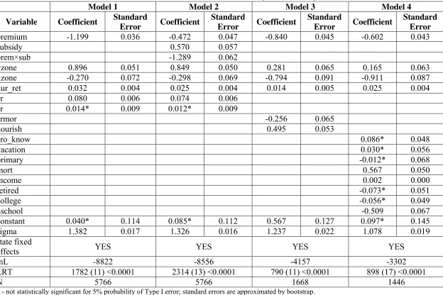
We report bootstrapped coefficients and standard errors for the Tobit coverage (3) model
in tables 5 and 6, employing high and low estimate of marginal insurance premium,
respectively. Each table includes 4 models, the first of which serves as a baseline and
includes marginal premium, indicators for the V and B/C/X flood zones, imputed asset
value, the hurricane return interval, and the historical average erosion rate (er) or
accretion rate (ar). Model 2 explores differences in coverage for subsidized
policyholders, while models 3 and 4 utilize survey data to explore the influence of local
hazard mitigation projects and household level variables, respectively. An asterisk
indicates covariates which are not statistically significant at the 5% level for a Type I
24
error. As models 1 and 2 utilize the full dataset, we deem these estimates more reliable
for covariates that are included in all models.
All coverage model specifications exhibit a negative flood insurance price
coefficient. Our estimates of price elasticity of demand are εp = -0.308 for the high
premium model and εp = -0.745 for the low premium model. Thus, both models indicate
inelastic demand, with the high premium providing an arguably better estimate and a
lower bound on the responsiveness of flood insurance demand to price. Models 2 explore
the variability in coverage by subsidy class. Subsidized policyholders are much more
price sensitive than non-subsidized, εp = -1.092 compared to εp = -0.330, respectively for
the high premium model (εp = -1.697 compared to εp = -0.366 for the low). Surprisingly,
these results also indicate that those households that face subsidized rates purchase less
flood insurance (marginal effect = -$44,100 (-$52,448) for the high (low) premium
model).
All coverage models indicate significantly higher insurance coverage in the
V-zone and lower insurance coverage in the B/C/X-V-zones relative to the A-V-zone. For
example, results from model 1, table 5 suggest that location within the V-zone increases
flood insurance coverage by $50,802, all else being equal, while location in the
B/C/X-zone decreases flood insurance coverage by $38,248. Of the models that utilize the full
dataset, the estimated marginal effect for V-zone ranges from $50,802 to $79,545; the
estimated marginal effect for X-zone ranges from -$38,248 to -$53,833. Estimated asset
value is statistically insignificant in all specifications, except for the fourth model (which
focuses on the sub-sample of survey respondents). Results from these models suggest
and 0.35%. The effect of hurricane return period is consistently negative in all coverage
models except one (in which it is statistically insignificant), suggesting that lower
hurricane risk is associated with lower flood insurance coverage. The estimated effect
ranges from -$2700 to -$3900 for a one-year increase in the return interval.
Results from models 1 suggest that those households facing higher erosion hazard
demand greater flood insurance coverage, with a marginal effect of around $3400 for one
foot increase in the erosion rate in each specification, though this effect is insignificant in
models 2. The rate of shoreline accretion has no statistically significant effect on flood
insurance demand. According to the results in models 3, community hazard mitigation
projects do not affect demand for flood insurance coverage. Models 4 explore the effect
of household-level factors on the demand for flood insurance. The income elasticity in
both models is around εI = 0.57, indicating flood insurance is a normal good. Those with
a mortgage hold much higher flood insurance coverage, with a marginal effect of $84,832
($78,069) in the high (low) premium model. Lastly, those with high school as their
highest level of educational attainment hold less flood insurance that those with graduate
level training (marginal effect around -$70,000).
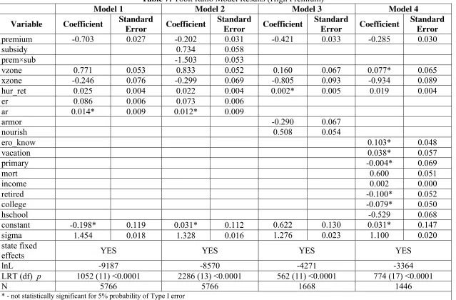
We turn next to the ratio models in tables 7 and 8, displaying parameter estimates
for the ratio of flood insurance coverage to estimated asset value using a single-censored
Tobit model (equation 3’). Again we find evidence of inelastic demand, on average, with
εp = -0.579 as a lower bound on responsiveness and εp = -0.826 as an upper bound. In
accord with the coverage models, subsidized policyholders exhibit elastic demand (εp =
-1.743 as a lower bound and εp = -2.459 as an upper bound), while non-subsidized
an upper bound). In contrast to the coverage models, subsidized policyholders exhibit
greater demand flood insurance when the dependent variable is expressed as a ratio
(marginal effect ranging from $0.333 - $0.379 per $1 asset value).
We find presence in the V flood-zone increases flood insurance coverage relative
to the A-zone. The marginal effect is $0.38 (between $0.44 and $0.57) per dollar of asset
value for the high (low) flood insurance premium models. Presence in lower flood risk
zones (B/C/X), on the other hand, diminishes flood insurance coverage by $0.12 - $0.19
per dollar of asset value (across both models). Flood insurance coverage is higher in
locations with higher erosion, though the effect is somewhat small ― $0.03 - $0.05 per
dollar asset value for each foot increase in the erosion rate. The coefficient for hurricane
return interval has an unexpected positive sign in the ratio models, possibly reflecting the
poor nature of this proxy for hurricane risk.
In contrast to the coverage models, flood insurance holdings are greater in
locations that manage coastal erosion through beach replenishment and lower in locations
that employ coastal armoring when demand is expressed as a ratio. Marginal effects for
both models indicate around $0.28 higher coverage per $1 asset value in communities
that employ beach replenishment and approximately $0.14 lower coverage per $1 asset
value in communities that utilize shoreline armoring. Results of model 4 lend further
support to the suggestion that mortgage status has a large impact on insurance coverage
(marginal effect ranging from $0.36 to $0.39 per $1 asset value). The income elasticity is
around 0.2 for both specifications. Flood insurance demand is lower for those with high
Discussion
Consistent with previous research, we find inelastic demand for flood insurance (U.S.
GAO 1983; Browne and Hoyt 2000; Kriesel and Landry 2004; Dixon et al. 2006). We
believe that our estimates may be more accurate than previous estimates due to the fact
that we employ marginal measures of insurance premium and utilize household-level
micro data. Our results, however, are limited to coastal properties in the southeast. Due
to the lack of information on deductible and replacement value, we estimate dual models
employing a high and low estimate of marginal premium for all specifications. Despite
this limitation our price elasticity estimates are rather tight; the overall estimate ranges
from -0.308 to -0.745. Estimates that employ the ratio of coverage to estimated asset
value also find evidence of inelastic demand, with εp ranging from -0.579 to -0.826. In
both cases, the former estimate is arguably better due to underlying assumptions.
Our results also provide some insight into the differences in coverage and
elasticity across subsidized and non-subsidized flood insurance policies. We find greater
price elasticity of demand for subsidized policyholders in both the coverage and ratio
specifications, ranging from -1.092 to -1.697 for the coverage models and from -1.743 to
-2.459 for the ratio models. In all models, price elasticity of demand for non-subsidized
policyholders is very low, ranging from -0.084 to -0.15 for the coverage models and from
-0.105 to -0.249 for the ratio models. In terms of raw coverage, subsidized policyholders
demand less coverage (ranging from -$44,100 to -$52,448) than non-subsidized
policyholders. When we examine demand as a ratio of coverage to asset value, however,
subsidized policyholder demand greater coverage (ranging from $0.333 to $0.379 per $1
market value of subsidized parcels, which should be older and more vulnerable to hazards
(since they were constructed before flood mitigation building standards were in force).
The Congressional Budget Office (Marron 2006) estimates that flood insurance
premium payments make up about 60% of the actuarial balance, leaving the general
taxpayer responsible for an estimated $1.3 billion per year. Our results support the
contention that moderate increases in flood insurance premiums will probably not induce
wholesale cancellation of policies, but the reduction in demand is likely to be
significantly greater for subsidized than non-subsidized policyholders. To the extent that
mortgage requirements mandate a specified level of flood insurance coverage, price
increases will have little effect on demand but will clearly induce negative welfare effects
on coastal households (assuming that the quality of post-disaster payouts and assistance
remains constant).25 Holding of a property mortgage induces the largest positive
marginal effects in our models ― on the order of $78,000 - $85,000 in the coverage
model and ranging from $0.36 - $0.39 per $1 asset value for the ratio model.
The efficacy of the mortgage requirement provision, however, has limits. The
raw data suggest that in 1998 only 39% of coastal properties were mortgaged. This likely
reflects a high level of wealth for many coastal property owners. The low proportion of
mortgages limits the influence of mandatory purchase provisions tied to mortgage status.
Moreover only 15% claim that they are required to hold flood insurance despite the
federal mandate for FDIC-backed mortgages. The raw data suggest that 11% of
respondents have allowed their flood insurance coverage to lapse as some time in the
past. This result is consistent with the suggestion that lenders have not been especially
25
zealous in enforcing insurance purchase requirements as required by law (Kunreuther
1984; Kunreuther 1996; Pasterick 1998), but anecdotal evidence suggests that more
recent data may not show a similar tendency.26 The subset of survey data providing
information on why those that have foregone flood insurance have made such a choice
indicates that subjective assessments of flooding tend to be lower than objective
estimates, as 55% of respondents claim that the price of insurance is too high or that the
risk of flooding is very low.
Our results provide some support for rational decision making with regard to
flood risk in the coastal zone. We find evidence of significantly higher insurance
coverage in the V-zone (ranging from $50,800 to $79,500 in the coverage models and
from $0.33 to $0.44 per $1 asset vale in the ratio models) and lower insurance coverage
in the Xzone (ranging from $38,200 to $53,800 in the coverage models and from
-$0.12 to -$0.19 per $1 asset vale in the ratio models) relative to the A-zone. This pattern
of results suggests that, conditional on the price of flood insurance and the value of the
asset at risk, homeowners anticipate higher damage and thus purchase greater coverage in
the 100-year flood zone with high velocity waves relative to the standard 100-year flood
zone, and that anticipation of damage and purchase of insurance coverage is lower in
flood zones with less risk. From the coverage models, we find flood insurance demand is
increasing in the estimated value of the asset at risk, but the effect is statistically
insignificant in most models (save for models 4, for which the estimated marginal effect
is between $100 and $200 dollars of coverage for a $1000 increase in asset value). Flood
26
insurance demand is increasing in hurricane risk, as reflected in the hurricane return
interval, for the coverage models. The marginal effect is between $2700 and $3900 for a
one year decrease in the hurricane return interval. This covariate, however, has a
counter-intuitive positive parameter in the ratio models. Thus, the result is not robust
across specifications.
We employ housing use data to test for wealth effects on flood insurance demand.
Our data include information on those households that use their coastal property as a
vacation home, as their primary residence, or as a rental unit. The rental market for
housing in coastal areas is typically very active. Those households that own multiple
homes (at least one in the coastal zone) and choose to forego rental income on their
coastal property are likely wealthier than those that supply in the rental market or those
for whom the coastal property is their primary residence. Neither the vacation home
dummy variable nor the primary residence dummy variable, however, proves to have any
explanatory power in our regression models. Thus, our findings are not particularly
insightful regarding wealth, and this remains a difficult topic to explore empirically.
Consistent with previous research (Browne and Hoyt 2000; Kriesel and Landry 2004) we
find a positive and statistically significant income elasticity in each model, around εI =
0.57 for the coverage model andεI = 0.22 for the ratio model.
The FEMA project that these data were collected for sought to explore the effect
of coastal erosion on the NFIP. The Flood Disaster Protection Act of 1973 made explicit
the terms under which damages due to coastal erosion would be indemnified under flood
insurance provisions. In particular, erosion losses must be associated with flooding
extent erosion risk affects expected loss and flood insurance demand. The data provide
some insight regarding the latter. We find that households facing higher erosion hazard
demand greater flood insurance coverage. The estimated marginal effects are on the
order of roughly $3300 per one foot increase in the annual historical erosion rate in the
coverage model (though the effect is statistically insignificant in model 2), and between
$0.03 and $0.05 per $1 asset value for each one foot increase in the erosion rate in the
ratio model. These results suggest that some homeowners view flood insurance as a form
of partial indemnification from erosion hazard. Moreover, those claiming knowledge of
the erosion rate at the nearest shore hold more flood insurance (around $0.06 per $1 asset
value) in the ratio model, while the effect of this covariate is statistically insignificant in
the coverage model. This result could point to an insurance demand effect that erosion
information has on coastal property owners, but, on the other hand, may simply reflect
correlation across insurance purchase and information attainment that reflects common
unobserved heterogeneity at the household level (i.e. risk-aversion).
Lastly, consistent with the findings of Kriesel and Landry (2004), we find some
evidence that community level erosion hazard mitigation projects influence flood
insurance holdings, but the effect is not consistently significant across model
specifications. Statistical significance is found only in the ratio models. For these
models, in contrast to the results of Kriesel and Landry, we find asymmetry across the
type of project, with shoreline armoring appearing to act as a substitute for flood
insurance (reducing coverage by around $0.15 per $1 asset value) and beach
replenishment appearing to act as a complement (increasing coverage by around $0.28
within the context of the Community Ratings System for hazard mitigation projects in
order to reduce their flood insurance premiums. The NFIP may be more inclined to
recognize and award credit for projects that are seen as complementary to flood insurance
holdings.
Conclusions
We use Tobit regression models to explore behavior and test theory regarding the
determinants of flood insurance coverage in the coastal zone using micro-level data for
nine southeastern U.S. counties. Unlike previous research, we incorporate both the
extensive and intensive margin of demand and employ measures of marginal insurance
premium to assess price elasticity. Overall estimates indicate price inelastic demand,
though subsidized policyholders are more sensitive to price and hold greater flood
insurance coverage (controlling for value of asset at risk).
We find support for rational choice in the coastal zone, with flood insurance
coverage correlated in the level of flood risk, controlling for insurance price and value of
the threatened asset. In one set of models, flood insurance demand is increasing in
hurricane risk, as reflected in the hurricane return interval, but this result is not robust
across specifications. The other set of models provide counter-intuitive results with
regard to hurricane risk, likely reflecting error in this county-level proxy for hurricane
risk. We attempt to proxy for household wealth, using dummy variable that reflect how
the owner uses the property, but results are statistically insignificant. We find a positive
and statistically significant income elasticity that is less than one indicating the flood
We find evidence that erosion risk does affect flood insurance demand, as
households facing higher erosion hazard demand greater insurance coverage and those
that claim knowledge of the erosion rate at the nearest shore hold more flood insurance.
Lastly, we find some evidence that community level erosion hazard mitigation projects
influence flood insurance holdings, with shoreline armoring appearing to act as a
substitute and beach replenishment appearing to act as a complement for flood insurance
in our ratio models. Unfortunately, we are unable to address the importance of “charity
hazard”, or a reliance on third-party assistance in the event of natural disaster. Finding
data that will allow for an assessment of charity hazard vis-à-vis other determinants of
References
Anderson, Dan R., 1974, The National Flood Insurance Program - Problems and Potential, Journal of Risk and Insurance, 41, 579-600.
Amemiya, Takeshi, 1973, Regression Analysis When the Dependent Variable is Truncated Normal, Econometrica, 41, 997-1016.
Amemiya, Takeshi, 1985, Advanced Econometrics, Harvard University Press, Cambridge, MA.
Baumann, Duane D. and John H. Sims, 1978, Flood Insurance: Some Determinants of Adoption, Economic Geography, 54(3), 189-96.
Browne, Mark J. and Robert E. Hoyt, 2000, The Demand for Flood Insurance: Empirical Evidence, Journal of Risk and Uncertainty, 20(3), 291-306.
Burby, Raymond J, 2001, Flood Insurance and Floodplain Management: the U.S. Experience, Environmental Hazards, 3, 111-22.
Casella, George, and Roger L. Berger, 2002, Statistical Inference, 2nd Edition, Duxbury-Thomson: Pacific Grove, CA.
Dixon, Lloyd, Noreen Clancy, Seth A. Seabury, and Adrian Overton, 2006, The National Flood Insurance Program’s Market Penetration Rate: Estimates and Policy
Implications, Report for the Federal Emergency Management Agency (contract # 282-98-0029), RAND Corporation: Santa Monica, CA.
Efron, B. and R. Tibshirani, 1986, Bootstrap Methods for Standard Errors, Confidence Intervals, and Other Measures of Statistical Accuracy, Statistical Science 1(1), 54-77.
Goldenberg, S.B., C.W. Landsea, A.M. Mestas-Nuñez, and W.M. Gray, 2001, The Recent Increase in Atlantic Hurricane Activity: Causes and Implications, Science
293, 474-8.
Guiso, Luigi and Tullio Jappelli, 1998, Background Uncertainty and the Demand for Insurance against Insurable Risks, The Geneva Papers on Risk and Insurance Theory, 23, 7-27.
Heinz Center for Science, Economics and the Environment, 2000, Evaluation of Erosion Hazards, final report to FEMA, contract EMW-97-CO-0375. Copies available at www.heinzctr.org
Krantz, David H. and Howard C. Kunreuther, 2007, Goals and Plans in Decision Making,
Judgment and Decision Making, 2(3), 137-168.
Kriesel, Warren, Alan Randall and Frank Lichtkoppler, 1993, Estimating the Benefits of Shore Erosion Protection in Ohio's Lake Erie Housing Market, Water Resources Research, 29(4), 795-801.
Kriesel, Warren and Craig Landry, 2004, Participation in the National Flood Insurance Program: An Empirical Analysis for Coastal Properties, Journal of Risk and Insurance, 71(3), 405-20.
Kunreuther, Howard, 1984, Causes of Underinsurance against Natural Disasters, The Geneva Papers on Risk and Insurance, 31, 206-20.
Kunreuther, Howard, 1998a, Introduction, in Paying the Price: The Status and Role of Insurance Against Natural Disasters in the United States, Kunreuther, Howard and Richard Roth (Eds.), Joseph Henry Press: Washington, D.C.
Kunreuther, Howard, 1998b, Insurability Conditions and the Supply of Coverage, chapter 2 in Paying the Price: The Status and Role of Insurance Against Natural
Disasters in the United States, Kunreuther, Howard and Richard Roth (Eds.), Joseph Henry Press: Washington, D.C.
Kunreuther, Howard and Mark Pauly, 2004, Neglecting Disaster: Why Don’t People Insure Against Large Losses? Journal of Risk and Uncertainty, 28(1), 5-21. Kunreuther, Howard, W. Sanderson, and R. Vetschera, 1985, A Behavioral Model of the
Adoption of Protective Activities, Journal of Economic Behavior and Organization 6, 1-15.
Lewis, Tracy, and David Nickerson, 1989, Self-Insurance Against Natural Disasters,
Journal of Environmental Economics and Management, 16, 209-23.
MacDonald, Don N., James C. Murdoch and Harry L. White, 1987, Uncertain Hazards, Insurance, and Consumer Choice: Evidence from Housing Markets, Land Economics, 63(4), 361-71.
Marron, Donald B, 2006, The Budgetary Treatment of Subsidies in the National Flood Insurance Program: Testimony before the Senate Committee on Banking, Housing, and Urban Affairs (January 25).
McClelland, Gary H., William D. Schulze, and Don L. Coursey, 1993, Insurance for Low-Probability Hazards: A Bimodal Response to Unlikely Events, Journal of Risk and Uncertainty, 7(1), 95-116.
Michel-Kerjan, Erwann and Carolyn Kousky, 2008, Come Rain or Shine: Evidence on Flood Insurance Purchases in Flordia, working paper, Wharton School, University of Pennsylvania.
Mossin, Jan, 1968, Aspects of Rational Insurance Purchasing, Journal of Political Economy, 76(4), 552-68.
Murphy, Kevin M., and Robert H. Topel, 1986, Estimation and Inference in Two-Step Econometric Models, Journal of Business and Economic Statistics, 3(4), 370-79. Nordhaus, W.D., 2006, The Economics of Hurricanes in the United States, American
Economic Association Annual Meetings: Boston, MA (January 6).
Palm, Risa, 1998, Demand for Disaster Insurance: Residential Coverage, chapter 3 in
Paying the Price: The Status and Role of Insurance Against Natural Disasters in the United States, Kunreuther, Howard and Richard Roth (Eds.), Joseph Henry Press: Washington, D.C.
Pasterick, Edward T., 1998, The National Flood Insurance Program, chapter 6 in Paying The Price: The Status and Role of Insurance Against Natural Disasters in the United States, Kunreuther, Howard and Richard Roth (Eds.), Joseph Henry Press: Washington, D.C.
Pricewaterhouse Coopers, 1999, Study of the Economic Effects of Charging Actuarial Based Premium Rates for Pre-FIRM structures I. Executive Summary.
Pricewaterhouse Coopers, Washington, D.C. (May 14).
Smith, Vernon L., 1968, Optimal Insurance Coverage, Journal of Political Economy, 76(1), 68-77.
Tobin, James, 1958, Estimation for Relationships with Limited Dependent Variables,
Econometrica, 26(1), 24-36.
Tobin, S. and C. Calfee, 2005, The National Flood Insurance Program’s Mandatory Purchase Requirement: Policies, Processes, and Stakeholders, American Institute for Research; Washington, D.C.
U.S. General Accounting Office (GAO), 1983, National Flood Insurance Program: Major Changes Needed if it is to Operate Without a Federal Subsidy, RCED-83-53, Washington, D.C. (January).
Wharton Risk Management and Decision Processes Center, 2008, Managing Large-Scale Risks in a New Era of Catastrophes, University of Pennsylvania: Philadelphia, PA.
Webster, P.J., G.J. Holland, J.A. Curry, and H.-R. Chang, 2005, Changes in Tropical Cyclone Number, Duration, and Intensity in a Warming Environment, Science, 309, 1844-6.
Table 1: Coastal Counties Included in Study
County Number in Sample
Percentage of Total
Survey Responses
(Rate)
Brazoria, Texas 488 0.080 121
(0.248)
Brevard, Florida 547 0.090 134
(0.245)
Brunswick, North Carolina 623 0.103 282
(0.453)
Dare, North Carolina 1069 0.176 564
(0.528)
Galveston, Texas 1124 0.185 423
0.376
Georgetown, South Carolina 493 0.081 193
(0.391)
Glynn, Georgia 326 0.054 68
(0.209)
Lee, Florida 455 0.075 129
(0.283)
Sussex, Delaware 949 0.156 178
(0.188)
Table 2: Insurance, Parcel, and Structure Descriptive Statistics
Variable Definition N Mean Std Dev
part* NFIP participation indicator 6074 0.521 0.569
flcov NFIP flood insurance coverage ($100) 5834 716.653 987.352
flratio NFIP flood insurance coverage / asset
value 5773 0.651 1.052
prem_hi Marginal flood insurance premium
(high) 6072 1.014 1.167
prem_lo Marginal flood insurance premium
(low) 6072 0.869 1.023
vzone* V flood zone indicator 6074 0.505 0.570
azone* A flood zone indicator 6074 0.410 0.561
xzone* X flood zone indicator 6074 0.085 0.318
postfirm* Indicator for structure built after FIRM 6074 0.627 0.551
subsidy* Indicator for subsidized insurance 6074 0.571 0.564
elev Elevation above base flood elevation
(BFE) 5882 3.305 15.751
brkaway* Indicator for breakaway walls present
below structure 6074 0.065 0.280
obstct* Indicator for obstructions present below
structure 6074 0.184 0.442
piles* Indicator for structure on piles 6074 0.689 0.528
crs Community Ratings System
classification (1998) 6072 8.346 1.475
er Erosion rate (feet/year) 6069 2.713 3.720
ar Accretion rate (feet/year) 6074 0.191 2.068
geotime number of years expected before
erosion reduces setback to zero 6074 787.924 8751.90
hur_ret Hurricane return interval (years) 6074 47.110 61.779
cbra* CBRA indicator 6074 0.056 0.263
distance Distance from the shore (feet) 6074 318.416 270.492
ocean* Oceanfront property indicator 6074 0.421 0.563
hp Housing sales price (1000s current $) 2844 187.177 669.815 asset_val Generated asset value (1000s current $) 6010 143.683 220.613
yearbuilt Year structure built 4632 1973.50 19.007
yearsold Year parcel sold 3740 1986.74 13.545
age_at_sale Age of structure when sold 6074 8.207 16.024
sqft Square footage 3947 2276.67 3142.42
vacant* indicator for vacant lot when sold 6074 0.540 0.568
dcbdm Distance from central business district
(m) 6074 4342.15 5801.51