An Algorithm to Determine RBFNN’s Center Based on the Improved Density Method

Open Journal of Applied Sciences, 2014, 4, 1-5

Published Online January 2014 in SciRes. http://www.scirp.org/journal/ojapps http://dx.doi.org/10.4236/ojapps.2014.41001

An Algorithm to Determine RBFNN’s Center

Based on the Improved Density Method

Mingwen Zheng, Yanping Zhang

School of Science, Shandong University of Technology, Zibo, China Email: [email protected], [email protected]

Received 26 September 2013; revised 1 November 2013; accepted 9 November 2013

Copyright © 2014 Mingwen Zheng, Yanping Zhang. This is an open access article distributed under the Creative Commons Attribution License, which permits unrestricted use, distribution, and reproduction in any medium, provided the original work is properly cited. In accordance of the Creative Commons Attribution License all Copyrights © 2014 are reserved for SCIRP and the owner of the intellectual property Mingwen Zheng, Yanping Zhang. All Copyright © 2014 are guarded by law and by SCIRP as a guardian.

Abstract

It takes more time and is easier to fall into the local minimum value when using the traditional full-supervised learning algorithm to train RBFNN. Therefore, the paper proposes one algorithm to determine the RBFNN’s data center based on the improvement density method. First it uses the improved density method to select RBFNN’s data center, and calculates the expansion constant of each center, then only trains the network weight with the gradient descent method. To compare this method with full-supervised gradient descent method, the time not only has obvious reduc-tion (including to choose data center’s time by density method), but also obtains better classifica-tion results when using the data set in UCI to carry on the test to the network.

Keywords

Radial Basis Function Neural Network; Data Center; Expansion Constant; Density Method; Full-Supervised Algorithm

1. Introduction

T Radial Basis Function Neural Network (RBFNN) is a forward neural network of good performance. It has faster learning rate than BP neural network and there is no local minimum problem. It can find the exact nonli-near system’s mapping as long as there are enough samples. So it is widely used like linonli-near approximation, data mining and image processing, etc.

determine the center of radial basis function [1-7]. Overall, the methods to determine the data center can be di-vided into two categories: supervised method and unsupervised method. In terms of supervised methods, it needs us to specify the number of the hidden layer. This requires some prior knowledge. But in most cases, we have only large amounts of data and we can’t clearly know their class. So it needs us to determine the centers to use the unsupervised method. In this paper, we proposed an improved density method—a dynamic clustering algorithm in mathematical statistics to select the data center of RBFNN and trained the weight value with gra-dient descent method. The simulation result is better.

This article is organized according to the following contents: Part 2 introduces the basic theory of RBFNN; Part 3 and Part 4 propose the specific algorithm; Part 5 is the experiments and analysis; Finally, conclusions.

2. The Basic Theory of RBFNN

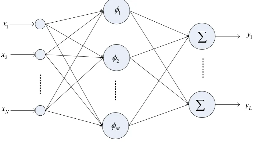
RBFNN is a three-layer feed-forward network, and it has only one hidden layer whose activation function is the radial basis function, for example, the Gauss function. Its output layer is a simple linear function. The network structure of RBFNN shown in Figure 1.

Let x_i∈RN,i=1, 2,,n is the i th- learning sample, each sample is N-dimensional, and then RBFNN’s

network output can be expressed by formula (1) and (2):

( )

(

)

(

)

1 1

, 1, 2, ,

M M

i i ik k k ik k k

k k

y f x w φ x c w φ x c i n

= =

= =

∑

=

∑

− =  (1)

(

)

exp

(

) (

2

)

T

k k

k k

k x c x c x c

φ

σ

 _{− −} 

 

− =

 

 

(2)

where yi is the network actual output according to the i th- learning sample; wik is the weight value of the i-th hidden layer node to the k-th output node;

k

φ is the Gauss Radial Function; ck is the k th- data center in the hidden layer; • represents the Euclidean distance; σk is the k th- width of the radial basis function.

[image:2.595.107.524.474.710.2]

Thus, RBFNN structure determination process is the process of seeking the three network parameters-w, c, σ. This paper determines the data center by the improved density method and its expansion constant and trains its weight value by gradient descent method.

Figure 1. The network structure of RBFNN.

1

x

2

x

N

x

1

y

L

y

1

φ

2

φ

M

φ

∑

3. The Original Density Method to Choose the Data Center of RBFNN

The Original density method is a dynamic clustering algorithm. It is different from the K-means clustering algo-rithm. The Samples is divided into M class in advance in K-means algorithm, and randomly select M data cen-ters. Then it calculates the Euclidean distance between each sample and each data center and the nearest sample will be classified as a class. Finally updates the cluster centers by different method. This method has obvious drawbacks. We don’t know how many data centers and don’t know their positions. However, the density method just need two value—d d1, 2

(

d1 <d2

)

, centre of sphere to each sample, d to be the sphere of radial, and the

number of samples falling within the sphere is called the density of this point. The maximum density of the sample is selected as the first cluster center, the second largest density of the sample as a candidate cluster cen-ters, then calculate the distance with previous cluster center. We don’t choose it as the cluster center if the dis-tance is less than d2, instead choose. And so on, we obtain some data centers of gradually smaller density and the

distance larger than d2 away from each other. The experience has shown that generally d2= ∗2 d1. Specific

steps are as follows:

Let sample set as

{

X i_i, =1, 2,,n

}

1) Given d d1, 2

(

d1<d2

)

,calculate the density-ρ for each sample, a deposit in set A, select the samples-ρmax

of the largest density to compose a group of cluster centers, and stored in set C;

2) Initialize classification. The Samples are classified according to minimum distance. Calculate the Eucli-dean distance between the remaining samples and the cluster center in set C and compare with d2: we classify as

a class of cluster center if the distance is less than d2 and instead is not classified. Thus, we obtain initial

classi-fication set B.

3) Modify category. To calculate the center of each cluster, go to (d) if the result is the same as origin cluster center. Otherwise, the center of each cluster is as new cluster center, go to 2)

4) Cluster is End. We obtain the finally cluster center set B. Store the element number of set B in M, and sig-nify c ii, =1, 2,,M as the cluster center vector.

Using the above steps, we obtained RBFNN hidden layer node number and center vectors, which the -thj data width is from literature [8], but we improved it as follow formula (3):

1,...,min,

j j i

i M i j c c

σ β

= ≠

= _ − (3)

where the parameter β is a constant greater or than equal 1 and can be appropriately selected in the experiment. Thus, we get all parameters of RBFNN.

4. The RBFNN’s Training Algorithm Based on Improved Density Method

4.1. Steps of Algorithm

Obtained the hidden layer structural parameters by Part 2 in this paper, we can get the RBFNN’s training algo-rithm based on improved density method. The steps are as follows:

1) We get the number M of hidden layer nodes, center vector c ii, =1, 2,,M and data width

, 1, 2, ,

j j M

σ = _{ by the algorithm in Part 2.}

2) Initialize the weight from hidden layer to output layer ωj and just optimize weight by the gradient descent method. The procedure is as follows:

a) Define the objective function, as follow formula (4)

2 1

1 2

n

i i

E e

=

=

∑

(4)

where n is sample number, ei is the error signal when we input the i th- sample. It is shown as follow formula (5):

( )

(

)

1

m

i i i i j i j

j

e d F X d ω G X c

=

= − = −

∑

− (5)

(

)

1

n

j i i j

i j E

e G X C

ω η η

ω =

∂

∆ = − = −

∂

∑

(6)

formula (7) of weight correction as shown below:

j j j

ω =ω + ∆ω (7)

c) Repeating process a), b) until the errors meet the requirements.

4.2. Analysis of Algorithmic Time Complexity

After the hidden layer parameters obtained can be intuitively seen from the above algorithm, we no longer train RBFNN’s centers and width, and weight training only. It is equivalent to linear optimization problems, the computation greatly reduced compared with the full-supervised learning algorithm. For the full-supervised learn-ing algorithm we need train weights, data centers, and the constant expansion of radial basis functions to learn at the same time. It is a very complicated nonlinear optimization problem. The specific analysis is as follows:

Assuming the total number of training sample is P, and we randomly select M1 data centers by the full-super-

vised algorithm and M2 by the improved algorithm proposed by this paper. When we use the full-supervised

al-gorithm, we need apply the formula (8), (9) and (6) to calculate data center, width and weight. The calculate amount is

1

3∗ ∗P M multiplication. But the calculate amount of the improved density method is

2 2

log_M

P∗ P+ ∗P M multiplication, which

2

log_M

P∗ P is the times that used to calculate the distance. That M1 and M2 is almost same. But the time to compute

2

log_M

P∗ P is less than P M∗ 1. So in theory, the time

complexity of the improved density method to train RBFNN is less than the full-supervised algorithm.

(

)

(

)

2 1

P j

j i i j i j

i j

c ηω e G X c X c

δ =

∆ =

∑

− − (8)

(

)

(

)

3 1

P j

j i i j i j

i j

e G X c X c

ω

δ η

δ =

∆ =

∑

− − (9)

(where, j=1M1).

5. Experiment and Analysis

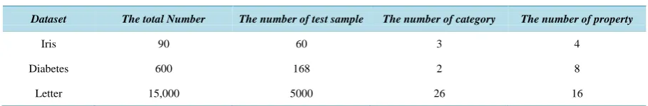
We use data sets Iris, Diabetes and Letter three datasets from UCI [9] to test the method on this article. The in-formation of data sets is shown in Table 1. We set Iris data set as an example. First we disarrange the data, and then classify to them and obtain data centers by the improved density method, and last train weight by the gra-dient descent method. The following are the specific parameters and experimental results.

Let d1= 10, d2=2 10. We reclassify the disarranged data and get 5 category by the density method. So

the network structure of RBFNN is identified as 4-5-1. Let β =0.5 when calculate the RBF center. Get the corresponding data width σ_j

(

j=15

)

by formula (3). Let the learning rate η=0.03 when train weight by the gradient descent method. Comparing with the full-supervised algorithm, the results are shown in Table 2

below:

The experiment environment is as follows:

[image:4.595.85.540.645.720.2]

CPU: dual-core, clocked at 1.83 GHZ; Memory: 1 GHZ; OS: Windows XP; Software: Matlab R2009a. As previous chapter 3.2 analysis, although the time complexity of two algorithm is both O(n2), the result of repeated testing shows the time-consuming of the improved algorithm is less than the full-supervised algorithm.

Table 1. Data sets of experiment.

Dataset The total Number The number of test sample The number of category The number of property

Iris 90 60 3 4

Diabetes 600 168 2 8

Table 2. Comparison of experiment results.

Iris Diabetes Letter

acc t(s) acc t(s) acc t(s)

Full-supervised algorithm 0.883 21.2363 0.844 38.2374 0.805 1860.33

The improved algorithm 0.942 19.2680 0.915 30.2623 0.882 1700.02

Note: acc stands for accuracy; The t(s) by the improved algorithm includes the time to compute data centers by the improved density method.

This confirms our previous analysis. When we test the letter dataset, 2 GB virtual memory settings on your computer does not meet the requirements. It leads the computer into the crash state. But it works well using of the improved algorithm.

6. Summary

This paper proposes an algorithm based on improved density method to choose data centers of RBFNN. Firstly, the density method is used to classify training samples and get the data centers, data width and category of data center. Then, we use these parameters to construct the RBFNN and then just train weight by the gradient descent method. It is equivalent to linear optimization problems. Finally, we obtain the RBFNN of better performance. However, the full-supervised learning algorithm is a very complex nonlinear optimization problem and it re-quires all parameters of RBFNN to learn simultaneously. So it is easy to make the result into the local minimum. In the classification of the three UCI datasets: Iris, Diabetes, and letter, the proposed algorithm obtains a better classification result.

References

[1] Chen, S., Cowan, C.F. and Grant, P.M. (1991) Orthogonal least squares learning algorithms for radial basis function networks. IEEE Transactions on Neural Networks, 2, 302-309. http://dx.doi.org/10.1109/72.80341

[2] Gomm, J.B. and Yu, D.L. (2000) Selecting radial basis function network centers with recursive orthogonal least squares training. IEEE Transactions on Neural Networks, 11, 306-314. http://dx.doi.org/10.1109/72.839002

[3] Han, M. and Guo, W. (2004) The full-supervised learning algorithm of radial basis function neural network. Chinese Journal of Science Instrument, 25, 454-457.

[4] Toh, K.-A. and Mao, K.Z. (2002) A global transformation approach to RBF Neural Network learning. Proceedings of

16th International Conference on Pattern Recognition (ICPR’02), 2, 96-99.

[5] Wei, H.K. and Ding, W.M. (2002) Dynamic method for designing RBF neural networks. Control Theory & Applica-tion, 19, 673-680.

[6] Wettschereck, D. and Dietterich, T. (1992) Improving the performance of radial basis function networks by learning center locations. Moody, J., Hanson, S. and Lippman R., Eds., Advances in Neural Information Processing Systems 4, Morgan Kaufmann Publishers, San Mateo.

[7] Tarassenko, L. and Roberts, S. (1994) Supervised and unsupervised learning in radial basis function classifiers. IEE Proceedings of Vision, Image and Signal Processing, 141, 210-216. http://dx.doi.org/10.1049/ip-vis:19941324 [8] Han, L.Q. (2006) Artificial neural network tutorial. Beijing University of Posts and Telecommunications Press, Beijing,

12Ver 1, 137.

[9] Web Site of UCI Machine Learning Repository. (2002) University of California, Irvine.