Dynamics importance sampling for the activation problem in
nonequilibrium continuous systems and maps
Stefano Beri
a, Riccardo Mannella
b, Peter V. E. McClintock
aa
Department of Physics, Lancaster University LA1 4YB, Lancaster, United Kingdom;
bDipartimento di Fisica, Universit`
a di Pisa Via Buonarroti 2, Pisa, Italy.
ABSTRACT
A numerical approach based on dynamic importance sampling (DIMS) is introduced to investigate the acti-vation problem in two-dimensional nonequilibrium systems. DIMS accelerates the simulations and allows the investigation to access noise intensities that were previously forbidden. A shift in the position of the escape path compared to a heteroclinic trajectory calculated in the limit of zero noise intensity is directly observed. A theory to account for such shifts is presented and shown to agree with the simulations for a wide range of noise intensities.
Keywords: Non Linear Dynamics, Non Equilibrium Systems, Numerical Simulations
1. INTRODUCTION
The study of stochastic processes in nonlinear systems is a very wide and important subject within modern physics as they are one of the main ways to describe the dynamics of a real system subject to a source of “noise”. If the noise intensity is small, the system is expected to spend the majority of its time in the close vicinity of some stable equilibrium point. Nevertheless, very rarely, a large fluctuation may drive the system far from the stable state, and eventually settle it in the basin of attraction of a different stable structure. As a result of this activation process, the qualitative dynamics of the system may change dramatically. Consider for example a vertical cavity surface emitting laser (VCSEL) operating with two stable linearly polarised modes; the random fluctuations due to spontaneous emission in the active medium may induce strong changes in the polarization resolved light intensity.1–4 In biological membranes, a current of ions passes through open ionic channels5 as the result of an activation process. Moreover, activation processes lie at the heart of many other physical phenomena in nonequilibrium systems, such as stochastic resonance,6directed diffusion in stochastic ratchets.7–9 The Kramers activation process lies within this class of problems.10–12 Despite its importance, the problem of activation cannot be regarded as solved. On the theoretical side, important steps toward the solution have been taken in the regime of zero noise intensity. It has been predicted that, even though the activation events become exponentially rare when the noise intensity approaches zero, they take place with increasing probability along activation trajectories that are close to an optimal trajectory. Such amost probable escape path(MPEP) can be obtained solving an auxiliary Hamiltonian system.13–20 The same picture still applies even for escape at short times (i.e. before quasi-equilibrium has been established).21 The solution of the escape problem using the MPEP is in principle true only for the limit of zero noise intensity. However, for real systems, the intensity of noise fluctuations is necessarily finite. More recently it has been established22 that finite noise diffusion does more than just changing the prefactor of the exponential. It causes the system to follow a path that differs from the zero-noise theoretical MPEP.
During the last years, in particular due to the availability of fast computers, the activation problem has also been extensively studied numerically, in particular using Monte Carlo simulations. However, even for simple systems, the simulation time grows exponentially with decreasing noise intensity. Consequently, the really interesting range of noise intensities, i.e. small enough for valid comparisons to be made with theoretical predictions, have in practice been inaccessible to numerical experiments. Intensive efforts are therefore being made to find ways of speeding up the simulations.23–25 The probability distribution for the system can be built
Further author information: send correspondence to Stefano Beri: [email protected] or to Riccardo Mannella: [email protected]
up iteratively23performing the simulation in regions far away from the equilibrium states. In this way, the shift of singularities in the probability distribution, and oscillation of the probability at the boundary due to finite noise intensity, have been observed. These features are consistent with the predicted shift of optimal paths due to the finiteness of the noise intensity. However, simulations able to reveal the predicted shift in the optimal path with increasing noise intensity are still lacking: to address this question we need numerical approaches which yield, not the probability distributions, but rather the actual paths followed by the dynamics of the system of interest. Simulation techniques based ondynamic importance sampling (DIMS) were proposed24 for 1-dimensional dynamical systems to study dynamics in the limit of very small noise intensity. DIMS aims to accelerate Monte Carlo integrations by adding an appropriately chosen biasing field to the equations of motion, which remain stochastic in nature. Standard techniques are then used to relate Monte Carlo results in the presence of the bias to the statistical observables of the original system.
The investigation of real systems (such as the lasers mentioned above) requires the analysis of higher dimen-sional nonequilibrium systems. However, the extension of DIMS to multidimendimen-sional systems is not straightfor-ward. An earlier biasing technique,25 introduced for both 1 and 2 dimensional systems, was found incapable of detecting either the shift of the escape path22 or saddle point avoidance,26 both of which had been predicted theoretically. Moreover, in the presence of singularities, a bad choice of bias might hide important physical features of the system of interest. Note that other numerical approaches, like the umbrella sampling technique27 are not appropriate for nonequilibrium systems.
The aim of this paper is the introduction of a generalized and robust version of DIMS valid, in principle for an arbitrary number of dimensions. Such an extended method would allow one to reveal the behaviour of the system in the vicinity of the MPEP in the finite noise regime. accelerating the simulation by exploitation of well-established zero-noise-limit theoretical results.
In order to give some concrete examples of the application of the technique, we apply it to the investigation of escape in three different multidimensional nonequilibrium systems: the inverted van der Pol oscillator, the harmonically driven overdamped Duffing oscillator and the polarization dynamics of a vertical cavity surface emitting laser. The noise intensities considered lie far beyond the range of anything investigated previously. As we will show, the predicted shift of the optimal path due to the finiteness of the noise is clearly resolved and turns out to be in excellent agreement with theory22over more than 4 orders of magnitude in the noise intensity. The extension of the algorithm to stochastic maps is discussed.
2. THEORY
As mentioned in the introduction, stochastic nonlinear systems are used to describe a very large number of different physical problems. In order to keep the discussion as general as possible, we consider a generic nonlinear system under the influence of noise described by the following Langevin equation
˙
x=f(x) +ξ(t), (1)
hξ(t)i= 0 hξ(t)ξ(s)i=ǫδ(t−s) (2)
Herexrepresents a vector of coordinates,f(x) is a nonlinear function, andξ(t) is a family of zero-mean uncor-related Gaussian noise processes of intensityǫ. The drift fieldf(x) is chosen in order to display multiple stable states (including eventuallyx→ ∞) and noise induced transitions between them are considered. For systems in detailed balance (for example iff(x) is the gradient of some potential function), activation takes place according to paths that are time-reversed relaxational trajectories.28 In what follows, we consider the case wheref(x) does not satisfy the detailed balance condition, and we will focus on the important case of coexisting steady states whose basins of attraction are separated by saddle cycles.
The time evolution of the probability density for the system (1) is regulated by the following Fokker-Planck equation
∂̺ ∂t =−
∂(f ̺)
∂x + ǫ
2
∂2̺
In the limit ǫ→0, (3) can be solved using the WKB expansion.13, 14 The probability distribution is considered to have the form
̺(x, t) =z(x, t) exp
−S(x, t)
ǫ
, ǫ→0, (4)
whereS(x, t) andz(x, t) are two functions. Inserting (4) in (3) and considering different order of expansion inǫ, at leading orderǫ−1 the auxiliary functionS turns out to be the solution of the Hamilton-Jacobi equation for a classical action
∂S ∂t =−H
x,∂S ∂x
. (5)
The Hamiltonian for the system,
H(x, p) = p 2
2 +p·f, (6)
is known as the Wentzell-Freidlin Hamiltonian14and the Hamiltonian equations for the system are
˙
x=f(x) +p, p˙=−pdf
dx. (7)
The evolution of the functionS along the solutions of (7) is calculated starting from dS dt =
∂S ∂t +
∂S
∂xx˙. Using ∂S ∂x
together with Eq.(5) and Eq.(6), the final equation for the action is
dS dt = 1 2p 2 . (8)
Being non-decreasing along trajectories and differentiable almost everywhere, the functionS can be considered as a non-equilibrium potential for the system.29–32 It is known from the theory of dynamical systems that S(x, t) can be a multi-valued function of position in the coordinate space.29, 31, 33, 34 In this case, more than one trajectory solution of (5) reaches the same point in coordinate space. In the limit ǫ → 0, only that of least actionSminis relevant, and all trajectories corresponding to higher values ofSare exponentially disadvantaged. Escape takes place along the least action trajectory with overwhelming probability in the limitǫ→0. This is the MPEP, and the action calculated along it is the “activation energy”. Regions of coordinate space reached by different families of optimal paths are separated by switching lines (SL).18, 19, 35 A trajectory ceases to be optimal after crossing a switching line. For this reason, the most probable escape path can touch the SL only asymptotically. Because the SL reaches the cycle asymptotically,18 the only possible optimal escape trajectories are heteroclinic paths connecting the initial state to the saddle cycle in infinite time.
To calculate the effect of finite, but small,ǫ6= 0 in this picture, a calculation of the next-to-leading order in the WKB expansion is performed. In this order of approximation, the prefactor z(x, t) satisfies.19
dz dt =−
∂fi ∂xiz−
1 2
∂2S
∂xi∂xiz (9)
where summation over repeated indexes is understood. The solution of (9) calls for a knowledge of the second derivatives of the action calculated along the characteristics. Differentiating twice (5), the following equations are obtained19
d dt
∂2S ∂xi∂xj
=− ∂
2H
∂xi∂xj − ∂2S ∂xi∂xk
∂2H ∂pk∂xj
− ∂
2S
∂xj∂xl ∂2H ∂xi∂pl −
∂2S ∂xj∂xl
∂2S ∂xi∂xk
∂2H
∂pk∂pl (10)
The non-constancy of the prefactor along the trajectories can be expressed in terms of a corrected non-equilibrium potential (dependent onǫ)
Sǫ=S−ǫlog(z). (11)
It is this corrected potential that has to be used to locate the position of the switching line for finite noise regimes. Points on the modified SL are defined byS1
the same point in the coordinate space.23 The modified switching line does not touch the cycle asymptotically, but hits it at a definite position which depends on the noise intensity. As a consequence, heteroclinic trajectories are no longer optimal and the optimal escape follows a path that differs from the MPEP.
The case of a non-linear stochastic map is very similar. Consider a generic map of the form
xn+1 =f(xn) +ξn, (12)
hξni= 0 hξnξmi=ǫδnm (13)
where the function f(x) is chosen to display multiple coexisting stable states. As (12) is a discrete system, a Fokker-Plank equation cannot be written for the probability distribution. Nevertheless, it has been proved36 that the MPEP for the map (12) satisfies the extended map
xn+1=f(xn) +λn, (14) λn+1 =
h
∂f ∂x
xn+1
i−1T
λn. (15)
Here the variableλn plays the role of the momentum pin (7) and the symbolT indicates the transpose matrix.
The “action” for the solutions of (14) and (15) can be calculated using the discrete version of (8)
Sn+1=Sn+ 1 2λ
2
n (16)
In the same way as in continuous systems, the transitions from an initial stable state to a final state take place along the path that minimize (16).
3. ALGORITHM
In this section we propose we propose an extension of DIMS24, 25to the multidimensional case. It will be used to unravel features of the topology close to the optimal escape path in the limit of small but finite noise intensity. The method is applicable to continuous systems or maps characterized by a stable attractor with a sizable basin of attraction, where escape takes place via a large fluctuation.
Consider a generic dynamical system of the form (1); we will focus on the transitions from a stable attractor
As toward a final saddle Fs. The process takes place in three steps: in the vicinity ofAs the dynamics of the
stochastic system is purely diffusive; then, when the system leaves the vicinity ofAs(the length scale is defined by √ǫ), the escape becomes essentially ballistic, along the MPEP and, in the vicinity of Fs, the finite noise diffusion dominates. In order to take into account the existence of these three regimes, the integration method is built as follow: the system is initially set close toAs, the exact equations of motion (1) are integrated using a standard SDE (stochastic differential equation) integrator: for the examples shown below, we used the Heun integrator.37 This reproduce the diffusive regime in the vicinity ofAs. We also set a boundary at some distance from the stable attractor: this boundary has nothing to do with the boundary of the basin of attraction, but it delineate where we define the diffusive regimes to change to ballistic. When the boundary is crossed, we switch from standard SDE integration to DIMS integration. Although the final result does not appear to depend on the boundary choice, nevertheless the boundary ought to be chosen on some rational basis: we require that the boundary should be fairly easily reached by the dynamical system when using straight SDE integration, but also that this event should not be too probable. In practice, a reasonable boundary could be e.g. a circle centered on the stable attractor, with a radius of a few√ǫ. This choice reproduces the diffusive dynamics in the vicinity of the stable state. When the system hits the boundary, we switch to the DIMS integrator: from the above discussion, we know that the SDE
˙
x=f(x) +ξ(t)
maps onto the Hamiltonian equation (7), so we switch to the integration of
˙
Ω
γ
x p
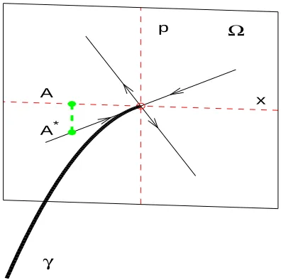
A
[image:5.595.197.395.72.269.2]A*
Figure 1. The scheme for one step of the DIMS method, where: Ω is a cross section in the extended phase space;γ(thick line) is the optimal path predicted by the theory; the thin lines are the stable and unstable eigenspaces (as indicated by the directions of the arrows) of the optimal path. The dashed lines represent respectively the coordinate spacexand the momentum space p. A is a point in the coordinate space,A∗is the corresponding point on the stable manifold of γ as
required by the integration procedure.
where p(x) is the momentum conjugated withx as obtained from the MPEP andξ(t) is the DIMS stochastic component. It is clear that in more than one dimension the probability of being exactly on the MPEP during each integration time step is negligible: but the idea is that we should nevertheless use in the integration of (17) the value of p(x) which “pulls” the escape tube toward the boundary. This is achieved by linearising the Hamilton equations near the MPEP, and using the p(x) that keeps the system on the stable manifold of the MPEP. A step of the scheme is explained in Fig.1. Consider a pointAin the coordinate space. The momentum
p(x) to be used in the equation (17) is calculated in the following way: the point A∗ in the extended phase space which has the same xcoordinate as A, and lies on the stable manifold of the MPEP, is located. The momentum of the pointA∗ is then used asp(x) in (17). The integration scheme is interrupted and reset if the trajectory leaves a small neighborhood of the MPEP (size of a few√ǫ). The generalization to stochastic maps is straightforward: once again it is necessary to define a boundary separating the diffusive region (in the vicinity of the initial stable state) and the ballistic region. Inside the diffusive region, Eq.(12) is integrated numerically in standard way; when the fluctuations bring the system in the ballistic region, the integration scheme switches to DIMS: instead of integrating directly Eq.(12), we integrate
xn+1=f(xn) +λn+ξn (18)
where the “momentum”λn is chosen in order to “pull” the path toward the MPEP. If the trajectory leaves a
neighborhood of the order of√ǫfrom the MPEP, it is rejected and the integration is restarted from scratch.
4. EXAMPLES
In this section we show some explicit examples of the application of the multidimensional DIMS algorithm. First, we consider the inverted van der Pol oscillator (IVDP). It is characterized by the presence of an unstable cycle with a stable point at its centre. DIMS is used here to study transitions from the stable state to the limit cycle. The IVDP system is described by the following pair of equations
˙
x=y
˙
y=−x−2η 1−x2
−3
−1
1
3
−3
−2
−1
0
1
2
x y
−3
−1
1
3
−3
−2
−1
0
1
2
[image:6.595.99.497.69.268.2]x y
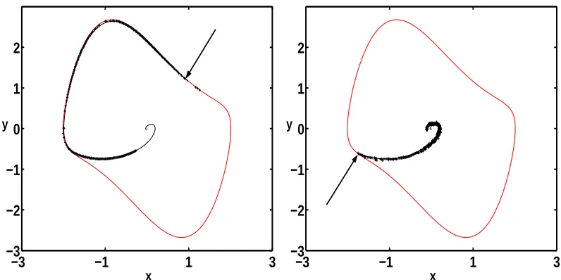
Figure 2. Comparison between theory and simulations for the escape in the IVDP system (19). Here the parameter η= 0.5 and two different noise intensities are considered: ǫ= 10−5
(left figure) andǫ= 10−2
(right figure). The limit cycle and the most probable escape path are indicated by full lines; the crosses are points on the ridge of the prehistory probability density for the escape. The arrows indicate the positions where the theoretical modified optimal escape path hits the cycle. The theory agrees well with the experimental points for both noise intensities. A significant shift in the position where the optimal path hits the boundary is evident.
Here xand y are dynamical variables and ξ(t) is a white Gaussian processes of unit intensity. The parameter
η determines both the friction and the pumping of energy in the system. The DIMS simulations have been performed for a range of intensities running between 10−5 and 10−2. Some results are shown in figure 2 for two different noise intensities. The agreement between the theoretical and experimental escape paths at finite noise intensities is seen to be excellent. The shift in the optimal path is continuous with the noise intensity and the change in the point where the MPEP hits the cycle is dramatic.
In order to show how the modified DIMS can be applied to non-autonomous stochastic systems we consider, as a second example, the harmonically driven overdamped Duffing oscillator
˙
x=x−x3+Asin (ωt) +√ǫξ(t). (20)
Here xis the dynamical coordinate,A andω are the amplitude and the frequency of the external driving, and
ξis a white Gaussian process of unit intensity. The driving termAsin (ωt) keeps the system out of equilibrium; the parametersAand ω are chosen to be in the non-perturbative, non-adiabatic regime. The dynamics of this system is characterized by two stable limit cycles separated by an unstable limit cycle. In the presence of noise, the system can fluctuate from one stable cycle to the other. Some simulation results are shown in Fig. 3. The experimental trajectory follows closely the heteroclinic path when it is far from the stable and unstable cycles. As the system approaches the unstable cycle, however, diffusion becomes important and the escape then runs along the finite noise escape path calculated using finite noise corrections. An increase in the noise intensity determines an increase in the shift of the hitting position of the experimental MPEP. Once again, the shift in the position is continuous with the noise intensity.
As a final example, we consider a noise-induced polarization switch in a VCSEL. If the linear dichroism of the active cavity and mirrors is small enough and the pumping is not too strong, the VCSEL emits in the fundamental transverse mode3, 4, 38and the polarization switches between two orthogonally polarized modes. In this regime, the polarization dynamics can be described using the polarization angleφand the ellipticityχ. The dynamical model for these is3
˙
0
5
10
15
−1
−0.5
0
0.5
[image:7.595.198.396.72.268.2]φ
x
Figure 3. Comparison of theory and simulations for the activation problem in the Duffing system (20). The parameters areA= 0.1 andω= 1. The noise intensity is hereǫ= 4×10⁻³. The dashed line indicate the steady states and the most probable escape path atǫ= 0. The solid line indicates the noise corrected optimal path. The crosses are points on the ridge of the prehistory probability density for the escape. The position where the noise corrected optimal path hits the saddle cycle is indicated by an arrow.
˙
φ = −ωlsin(2χ)
cos(2χ)cos(2φ) +γl sin(2φ)
cos(2χ)−ωnsin(2χ) +ξφ(t) (22)
hξχ(t)i = hξφ(t)i= 0 ∀t (23)
hξχ(t)ξχ(s)i = hξφ(t)ξφ(s)i=ǫδ(t−s) hξφ(t)ξχ(s)i= 0 ∀t, s (24)
Here ωl and γl are the dispersive (birefringence) and absorptive (dichroism) linear anisotropies, and γn and ωn =αγl (αis the linewidth enhancement factor) are the nonlinear anisotropies. The spontaneous emission of photons in the cavity is described by the Gaussian stochastic variablesξχandξφ. The dynamical variableχmay vary between −π
4 and π
4 and the angleφmay vary between 0 and π. With a proper choice of the parameters, two linear polarization modes are stable: the ˆx-polarized mode (corresponding to χ = 0 and φ = 0) and the ˆ
y-polarized mode (corresponding toχ= 0 andφ= π
2). Their basins of attractions are separated by an unstable limit cycle similar to the one in IVDP system.
The DIMS scheme has been applied here to investigate the transitions from the ˆy-polarized mode to the limit cycle. In figure 4 the numerical simulations are compared with the theoretical MPEP for different values of the noise intensity. As expected, when the noise intensity increases, the simulations follow the MPEP less closely and they leave the basin of attraction of the initial lasing mode earlier.
5. CONCLUSIONS AND DISCUSSION
−10 −5 0 5 10 15 −0.8
−0.4 0 0.4 0.8
(a)
ε = 2E−6
t χ
−10 −5 0 5 10 15
−0.8 −0.4 0 0.4 0.8
(b)
ε = 9E−6
[image:8.595.100.494.71.267.2]t χ
Figure 4. Comparison between theory and simulations for the polarization switches in a VCSEL. The noise intensity changes from (a) to (b); the dashed lines are the theoretical MPEP and the solid lines are the results of the simulation. The full circle marks the point where half of the trajectories plus one leave the basin of attraction of the initial lasing mode. The shift of this point with the noise intensity is evident.
in this paper. The technique provides a way of extending experimental studies to noise intensities that were previously inaccessible, and promises to accelerate research in many fields of science, e.g. in the investigation of the polarization of flip dynamics in vertical cavity surface emitting lasers or in the motion of ions in the pores of cellular membranes. The discrete version of the algorithm may be used as a tool to investigate problems in laser dynamics.39, 40
ACKNOWLEDGMENTS
We are grateful for valuable discussions with Dmitri Luchinsky and Stanislav Soskin. The research has been supported in part by the Engineering and Physical Sciences Research Council (UK) and by INTAS.
REFERENCES
1. M. B. Willemsen, M. P. van Exter, and J. Woerdman, “Anatomy of a polarization switch of a vertical-cavity semiconductor laser,”Phys. Rev. Lett 84, pp. 43377–4340, 2000.
2. M. B. Willemsen, M. P. van Exter, and J. P. Woerdman, “Correlated fluctuations in the polarization modes of a vertical cavity semiconductor laser,”Phys. Rev. A60, pp. 4105–4205, 1999.
3. M. P. van Exter, R. F. M. Hendriks, and J. P. Woerdman, “Physical insight into the polarization dynamics of semiconductor vertical-cavity lasers,”Phys. Rev. A57, pp. 2080–2090, 1998.
4. M. P. van Exter, M. B. Willemsen, and J. P. Woerdman, “Polarization fluctuations in vertical-cavity semi-conductor lasers,”Phys. Rev. A58, pp. 4191–4205, 1998.
5. R. S. Eisenberg, M. M. Klosek, and Z. Schuss, “Diffusion as a chemical-reaction - stochastic trajectories between fixed concentrations,”J. Chem. Phys.102, pp. 1767–1780, 1995.
6. M. I. Dykman, D. G. Luchinsky, R. Mannella, P. McClintock, N. D. Stein, and N. G. Stocks, “Stochastic resonance in perspective,”Nuovo Cimento D17, pp. 661–683, 1995.
7. F. A. F. Julicher and J. Prost, “Modeling molecular motors,”Rev. Mod. Phys. 69, pp. 1269–1281, 1997. 8. M. O. Magnasco, “Forced thermal ratchets,”Phys. Rev. Lett.71, pp. 1477–1481, 1993.
10. H. Kramers, “Brownian motion in a field of force and the diffusion model of chemical reactions,” Physica
7, pp. 284–304, 1940.
11. V. I. Mel’nikov, “The Kramers problem: fifty years of development,”Phys. Rep.209, pp. 1–71, 1991. 12. M. I. Dykman, “Large fluctuations and fluctuational transitions in systems driven by colored Gaussian
noise–a high frequency noise,”Phys. Rev. A42, pp. 2020–2029, 1990.
13. D. Ludwig, “Persistence of dynamical systems under random perturbations,”SIAM Rev.17, pp. 605–640, 1975.
14. M. Freidlin and A. D. Wentzel, Random Perturbations in Dynamical Systems, Springer, New York, 1984. 15. R. S. Maier and D. L. Stein, “Effect of focusing and caustics on exit phenomena in systems lacking detailed
balance,”Phys. Rev. Lett.71, pp. 1783–1786, 1993.
16. R. S. Maier and D. L. Stein, “How an anomalous cusp bifurcates in a weak-noise system,” Phys. Rev. Lett.
85, pp. 1358–1361, 2000.
17. M. I. Dykman, M. M. Millonas, and V. N. Smelyanskiy, “Observable and hidden features of large fluctuations in nonequilibrium systems,”Phys. Lett. A195, pp. 53–58, 1994.
18. V. N. Smelyanskiy and M. I. Dykman, “Topological features of large fluctuations to the interior of a limit cycle,”Phys. Rev. E55, p. 2516, 1997.
19. R. S. Maier and D. L. Stein, “A scaling theory of bifurcations in the symmetrical weak-noise escape problem,” J. Stat. Phys.83, pp. 291–357, 1996.
20. J. Lehmann, P. Reimann, and P. Hanggi, “Surmounting oscillating barriers: path-integral approach for weak noise,”Phys. Rev. E62, pp. 1639–1642, 2000.
21. S. M. Soskin, V. I. Sheka, T. L. Linnik, and R. Mannella, “Short time scales in the Kramers problem: A stepwise growth of the escape flux,”Phys. Rev. Lett.86, pp. 1665–1669, 2001.
22. A. Bandrivskyy, S. Beri, and D. G. Luchinsky, “Noise-induced shift of singularities in the pattern of optimal paths,”Phys. Lett. A 314, pp. 386–391, 2003.
23. A. Bandrivskyy, S. Beri, D. G. Luchinsky, R. Mannella, and P. McClintock, “Fast Monte Carlo simulations in the probability distributions of nonequilibrium systems,”Phys. Rev. Lett.90, p. 210201, 2003.
24. D. M. Zuckermann and T. B. Woolf, “Efficient dynamic importance sampling of rare events in one dimen-sion,”Phys. Rev. E63, p. 016702, 2001.
25. T. B. Woolf, “Path corrected functionals of stochastic trajectories: towards relative free energy and reaction coordinate calculations,”Chem. Phys. Lett.289, pp. 433–441, 1998.
26. D. G. Luchinsky, R. S. Maier, R. Mannella, P. V. E. McClintock, and D. L. Stein, “Observation of saddle-point avoidance in noise-induced escape,”Phys. Rev. Lett.82, pp. 1806–1809, 1999.
27. C. Dellago, P. G. Bolhouis, F. S. Csajka, and D. Chandler, “Transition path sampling and the calculation of rate constants,”J. Chem. Phys.108, pp. 1964–1977, 1998.
28. D. G. Luchinsky and P. V. E. McClintock, “Irreversibility of classical fluctuations studied in analogue electrical circuits,”Nature389, pp. 463–466, 1997.
29. R. Graham and T. Tel, “Existence of a potential for dissipative dynamical systems,”Phys. Rev. Lett. 52, pp. 9–12, 1984.
30. R. Graham and T. Tel, “Weak noise limit of fokker-planck models and nondifferentiable potentials for dissipative dynamical systems,”Phys. Rev. A31, pp. 1109–1122, 1985.
31. H. R. Jauslin, “Nondifferentiable potentials for nonequilibrium steady states,”Physica A144, pp. 179–191, 1987.
32. R. Graham, “Macroscopic potentials, bifurcation and noise in dissipative systems,” in Noise in Nonlinear Dynamical Systems, F. Moss and P. V. E. McClintock, eds.,1, pp. 225–278, Cambridge University Press, 1989.
33. V. Arnold, Mathematical Methods of Classical Mechanics, Springer-Verlag, Berlin, 1978.
34. M. V. Day, “Recent progress on the small parameter exit problem,”Stochastics20, pp. 121–150, 1987. 35. M. I. Dykman, P. V. McClintock, V. N. Smelyanskiy, N. D. Stein, and N. G. Stocks, “Optimal paths and the
prehistory problem for large fluctuations in noise driven systems,”Phys. Rev. Let.68(18), pp. 2718–2721, 1992.
37. R. Mannella, “Integration of stochastic differential equations on a computer,” Int. J. Mod. Phys C 13, pp. 1177–1194, 2002.
38. M. P. van Exter, A. Al-Remawi, and J. P. Woerdman, “Polarization fluctuations demonstrate nonlinear anisotropy of a vertical-cavity semiconductor laser,”Phys. Rev. Lett.80, pp. 4875–4878, 1998.
39. V. A. Gaisyonok, E. V. Grigorieva, and S. A. Kashchenko, “Poincar´e mappings for targeting orbits in periodically driven lasers,”Opt.Commun.124, pp. 408–417, 1996.