THE DESIGN OF FUZZY LOGIC CONTROLLER VIA COPYING A LINEAR CONTROLLER

(1)

A Monthly Double-Blind Peer Reviewed Refereed Open Access International e-Journal - Included in the International Serial Directories.

GE-International Journal of Engineering Research

112 | P a g e

THE DESIGN OF FUZZY LOGIC CONTROLLER VIA COPYING A LINEAR CONTROLLER

Ibekwe B.E.Ph.D

Department of Electrical and Electronic Engineering Enugu State University of Science and Technology (ESUT)

Ilo Frederick U.Ph.D

Department of Electrical and Electronic Engineering Enugu State University of Science and Technology (ESUT)

Eneh Princewill Chigozie

Department of Electrical and Electronic Engineering, Enugu State University of Science and Technology, Enugu Nigeria

Abstract

The design of the fuzzy logic controller via copying a Linear Quadratic Regulator (LQR) is presented. To synthesize a fuzzy controller, we pursued the idea of making it match the LQR for small inputs since the LQR was so successful[9]. Then we still have the added tuning flexibility with the fuzzy controller to shape the control surface so that for larger inputs, it can perform differently from the LQR. The 25 “If-Then” rules determined heuristically based on the knowledge of the plant dynamics were stored in the MATLAB workspace from where they were transferred into the fuzzy controller model ready to be used for simulation in MATLAB/Simulink environment.

Keywords: Fuzzy controller, LQR, tuning flexibility, synthesized controller, If-Then rules.

1.0 INTRODUCTION

Fuzzy controller can be viewed as an artificial decision maker that operates in a closed loop

system in real time (see fig. 1.1). It gathers the plant output data y(t), compares it with the

reference input r(t) and decides on what the plant input u(t) should be to ensure the

performance objectives are met. Note that every fuzzy control system is a nonlinear system

and more so that even if the plant is linear, fuzzy and hence fuzzy control is nonlinear.

To design the fuzzy controller, the control engineer must gather enough information on how

artificial decision maker should act in a closed-loop system. Sometimes, this information

could come from a human decision maker (the machine operator), who performs the control

task, while at other times, it may come from the control engineer who comes to understand

the plant dynamics and write down a set of rules about how to control the system without

outside help[7].

GE-International Journal of Engineering Research

Vol. 4, Issue 7, July 2016 IF- 4.721 ISSN: (2321-1717)

© Associated Asia Research Foundation (AARF) Publication

(2)

GE-International Journal of Engineering Research

113 | P a g e

These “rules” basically say, “If the plant output and reference input are behaving in a certain

manner then the plant input should be some value.” A whole set of such “If-Then” rules are

loaded into the rule base and inference strategy is chosen, then the system is ready to be

[image:2.595.97.507.110.237.2]

tested to see if the closed-loop specifications are met.

Fig. 1:1 Fuzzy Controller Architecture[9].

1.1 Conventional/Fuzzy Control Approach to Balancing Control

There is no general systematic procedure for the design of fuzzy controllers that will

definitely produce a high performance fuzzy control system for a wide variety of application.

It is necessary to learn about fuzzy controller design via example[9]. Although, numerous

linear control design techniques have been applied to this particular system, here we consider

the performance of only the LQR. The objective is of two folds:[8]

i. To form a base line for comparison of fuzzy control design to follow.

ii. To provide a starting point for the synthesis of fuzzy controller.

A linear map such as LQR can be easily approximated by a fuzzy system (at least for small

values of inputs to the fuzzy system). For the fact that a linearized system is completely

controllable and observable, linear state-feedback strategies, such as LQR is applicable. The

performance index for the LQR is given by[5],

J = X_(t)T _Qx

(t)+ U(t)T Ru(t) dt ∞

o (1.1)

Where Q and R are the weighting matrices of appropriate dimension corresponding to the

state X and input U respectively. Given a fixed Q and R, the feedback gains that optimize the

function J can be uniquely determined by solving an algebraic Riccati equation in MATLAB.

In effect, the idea of using the LQR controller is analogous to the actual implementation o f

results for the case where there is no additional load or mass to the end point (i.e. nominal

case) in a pendulum. Now, when an extra weight or sloshing liquid (using a watertight bottle)

is attached to the end point of the pendulum, for instance, the performance of all the linear Inference

mechanism

Rule base efuz_D

zi

fi

ca

ti

on

Fuzzi

fi

ca

ti

on

Process

(3)

GE-International Journal of Engineering Research

114 | P a g e

controller degrades considerably, often resulting in unstable behaviour, and here a fuzzy

control is needed[7].

2.0 DESIGN Assumptions:

The following assumptions were made during the design[7]:

i. Assume that all the input universes of discourse have uniformly distributed triangular

membership functions (as shown in fig. 2.1) with the effective universes of discourse,

all given by (-1, +1) i.e. so that the left-most membership function and the right-most

membership function saturate at -1 and +1 respectively.

ii. Assume we label the membership functions with linguistic numeric indices that are

integers with zero at the middle.

iii. Assume an isolated power station with the following parameters (see table 2.1).

(a) (b)

[image:3.595.86.456.495.687.2]

Fig. 2.1: Set of input membership functions[9].

Table 2.1: Parameters for an Isolated Power Station[5]

Gain Time Constant

Turbine KT = 1

Governor Kg = 1

Amplifier KA = 10

Exciter KE = 1

Generator KG = 0.8

Sensor KR = 1

Inertia H = 5

Regulation R = 0.05

γr = 0.5

γg = 0.2

γA = 0.1

γE = 0.4

γG = 1.4

γR = 0.05

Assume a sudden load change of PL = 0.2 (p.u). E1−3 E2−2 E1−1 1 E₁0 E₁+1 E1+2 E1+3

-5.1 -3.4 -1.7 0 1.7 3.4 5.1 i(rad)

E2−3 E2−2 E2−1 1 E₂0 E₂+1 E2+2 E2+3

(4)

GE-International Journal of Engineering Research

115 | P a g e

2.1 METHODOLOGY

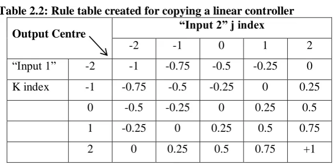
2.1.1 Summation Operation

First, the IF – THEN rules were arranged so that the output membership function centres are

equal to a scaled sum of the premise linguistic numeric indices. For a fuzzy controller in

general, the centre of the controller output is given by[9]:-

Y = j + k … + l x _{N−1 n}2 (2.1)

Where Y is the value of the output membership function centres (j + k … + l) are sum of the

premise linguistic numeric indices

N is the number of the membership functions in each input universe of discourse.

n is the number of inputs as assumed by the designer.

If for instance,

j + k = sum of the premise linguistic numeric indices

N = 5 (as a standard)

n = 2

Substituting the above values, equation 2.1 reduces to:

Y = j + k x _{5−1 2}2 (2.2)

= (j + k)1 4

[image:4.595.74.417.496.668.2]

Equation 2.2 was then used to generate the rule base shown in table 2.2

Table 2.2: Rule table created for copying a linear controller

Output Centre “Input 2” j index

-2 -1 0 1 2

“Input 1” -2 -1 -0.75 -0.5 -0.25 0

K index -1 -0.75 -0.5 -0.25 0 0.25

0 -0.5 -0.25 0 0.25 0.5

1 -0.25 0 0.25 0.5 0.75

2 0 0.25 0.5 0.75 +1

Observations:

 From table 2.2, it can be seen that the fuzzy system is normalized i.e. the effective

(5)

GE-International Journal of Engineering Research

116 | P a g e

 Again, the body of the table represents the centres of nine distinct output membership

function centres.

 Note the diagonal of zeros; and by viewing the body of the table as a matrix, we see

that it has a certain symmetry to it. This symmetry is not by accident but a

representation of abstract knowledge about how to control the system[7].

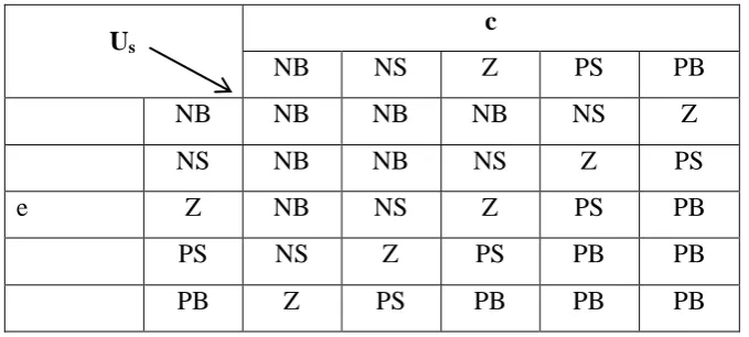
Table of Linguistic Variable with Rules:

The linguistic variables were written from the output membership function centres of table

[image:5.595.79.419.284.437.2]

2.2. Hence, we have table 2.3 as shown.

Table 2.3: Showing the Linguistic Variables (Us = output membership function centres;

e = error and c = change in error)

Us

c

NB NS Z PS PB

NB NB NB NB NS Z

NS NB NB NS Z PS

e Z NB NS Z PS PB

PS NS Z PS PB PB

PB Z PS PB PB PB

The output membership function centres are 25 in number, and these represent 25 IF-THEN

rules from this table. These 25 rules were clearly spelt and stated, and then stored in the

MATLAB workspace from where they were transferred into the fuzzy controller by opening

its dialog box. Here are some of the IF-THEN rules organized from the rule table:-

IF e is negative big NB and c is negative big NB, THEN Us is negative big NB. IF e is

negative small NS and c is negative big NB THEN Us is negative big NB. IF e is zero Z and c

is negative big NB THEN Us is negative big NB. IF e is positive small PS and c is negative

big NB THEN Us is negative small NS. IF e is positive big PB and c is negative big NB

(6)

GE-International Journal of Engineering Research

117 | P a g e

2.1.2 The Scaling Gain

Having achieved so far in the design, next is to pick the scaling gains so that the fuzzy system

implements a weighted sum. Prior to this, the LQR was first designed by solving its algebraic

Riccati equation in MATLAB[5], thus:

Given performance index J = (_o∞ X₁2+ 5x₃2+ U2) dt (2.3)

The state equation in matrix form[5] is given by

∆Pv ∆Pm

∆ω =

−1

𝛾𝑔 0 −1 Rγg 1

γT 1 γT 0

0 _2H1 −D_2H

∆Pv ∆Pm ∆ω + 0 0 −1 2H

∆PL+ 1 γg

0 0

∆Pref (2.4)

Substituting the parameter values of the system (see the third assumption) into the state

equation (2.4), with∆P_ref = 0 we have:

x = −5 0 − 1002 − 2 0 0 0.1 − 0.08

x + 00 −0.1

U (2.5)

and the output equation y = [0 0 1] x (2.6)

where y = ∆ω and x =

∆Pv ∆Pm

∆ω

 For this system we have by inspection:

A = −5 0 − 1002 − 2 0 0 0.1 − 0.08

, B = 00

−0.1

, C = 0 0 1 , Q = 1 0 00 0 0 0 0 5

and R = 1

To obtain the optimal feedback gain vector to minimize the given performance index (eqn.

2.3), we use the following, MATLAB commands[8]:-

PL = 0.2;

A = [-5 0 -100; 2 -2 0; 0 0.1 -0.08];

B = [0; 0; -0.1]; BPL = PL * B;

C = [0 0 1]; D = 0;

(7)

GE-International Journal of Engineering Research

118 | P a g e

Q = [1 0 0; 0 0 0; 0 0 5];

R = 1;

[K, P] = Lqr2 (A, B, Q, R)

Af = A – B * K

t = 0 : 0.02 : 1;

[y, x] = Step (Af, BPL, C, D, 1, t);

Plot (t, y), grid, xlabel („t, sec‟), ylabel („pu‟)

The result is

K1, K2, K3 respectively

= 0.0834, -0.2875, -12.1381

P

= 0.1100 0.0267 -0.8338

0.0267 0.1231 2.8751

-0.8338 2.8751 121.3810

Af

= -5.0000 0 -100.0000

2.0000 -2.0000 0

(8)

GE-International Journal of Engineering Research

119 | P a g e

Fig. 2.2: Plot of frequency deviation responses

[image:8.595.108.490.39.324.2]

The simulation block diagram of the system condition is constructed as shown in fig. 2.3

Fig. 2.3: Simulation Block Diagram of the System[5].

The state-space description dialog box was opened and the values of A, B, C and D constants

were entered in the appropriate box in Matlab matrix notation. +

- x = A_{y = C}x + Bu

x + Du Demux

K

PL

Step



Scope Feedback gain

using LQR design

(9)

GE-International Journal of Engineering Research

120 | P a g e

2.1.3 Choice of Scaling Gains

To choose the scaling gains so that the fuzzy system implements a weighted sum, the

appropriate gain on the ith input-output pair is gigo; so to copy the ki of the state feedback

controller, we choose[9]:-

gigo = ki (2.7)

Where ki = optimal gain of LQR

gi = ith input gain

go = ith output gain

Choosing the controller input that most greatly influences the plant behaviour to be g3 = 2[9](2.8)

From the results of the optimal gains calculated, K3 = -12.14.

g3g0 = K3 from equation (2.7) and hence, 𝐾3

𝑔3 = 𝑔0

∴ 𝑔0 =

−12.1381

2 = −6.069

Now, for 𝑔₀ = -6.07, the input gains are:

𝑔₁ = 0.0834_−6.07 = −0.01374

𝑔₂= −0.2875

−6.07 = 0.04736

𝑔₃= −12.138

−6.07 = 1.9996 ≅ 2

Try the scaling gains of 0.04736 or 2.

3.0 ANALYSIS RESULT

The gains of 2 were chosen so that the fuzzy system implements a weighted sum and is

inserted in any model bearing the fuzzy controller and any chosen compensator. A simulation

is done in Matlab/Simulink environment to get a result.

4.0 CONCLUSION

Fuzzy logic is dynamic because human expert has the responsibility to control the plant; and

(10)

GE-International Journal of Engineering Research

121 | P a g e

model in problem solving, it is a natural language and easy to understand. Above all, it acts as

a supplementary controller to major controllers in a given system.

REFERENCES

1) Berde, M.A. (2000). Thyristor Control Engineering (Power Electronics), 9th Edition, Khama Publishers.

2) Duber, G.K. (1998). Power Semiconductor Controlled Drive, Prentice Hall Int.

3) Harish, C.R. (1999). Power Electronics, 3rd Edition, Galgotia, New Delhi.

4) Holt, J. and Schwellenberg, U. (1983). A New Fast Response Current Control Scheme for Line Controlled Converters. IEE Transaction on Industrial Appl. Vol. 1A-19, No. 4, July, pp. 127-134.

5) HadiSaadat (2004). Power System Analysis, 2nd Edition, McGraw Hill Publication.

6) Ibekwe, B.E. et al (2014). Guiding Principles in Selectinga.c to d.c Converters for Power Factor Collection in a.c Transmission System, IJERA Publications.

7) Ibekwe, B.E. (2016). Ph.D Thesis on Dynamic Compensation of Reactive Power in 330kv Transmission Line using Fuzzy Controller Static Var Compensator, ESUT Enugu (unpublished).

8) PrabhaKundur (2010). Power System Stability and Control, Tata McGraw Hill Edition.

9) Passino and Yurkovich (1998). Fuzzy Logic Control, Addison Wesley Longman Inc.