International Research Journal of Mathematics, Engineering and IT Vol. 3, Issue 6, June 2016 IF- 3.563 ISSN: (2349-0322)
© Associated Asia Research Foundation (AARF)
Website: www.aarf.asiaEmail : [email protected] , [email protected]HAAR WAVELET METHOD FOR THE SOLUTION OF TWO-DIMENSIONAL PARABOLIC PARTIAL DIFFERENTIAL EQUATIONS
Sumana R. Shesha1, Tejuswini M.2 and Achala L. Nargund3
1,2,3P. G. Department of Mathematics and Research Centre in Applied Mathematics
M. E. S. College of Arts, Commerce and Science,15th cross, Malleswaram, Bangalore - 560003.
ABSTRACT
Parabolic partial differential equations arise in the mathematical modelling of many physical
phenomena. In this paper, we use Haar wavelet method for the numerical solution of
two-dimensional heat equation. The basic idea of Haar wavelet collocation method is to convert
the partial differential equation into a system of algebraic equations that involves a finite number
of variables. The numerical results are compared with the exact solution to prove the accuracy of
the Haar wavelet method.
Keywords:
Parabolic partial differential equations, two-dimensional heat equation, Haar wavelets, collocation points.Mathematics Subject Classification:
65T601 Introduction
Parabolic partial differential equations (PDEs) are used to describe variety of problems in science
including heat diffusion, ocean acoustic propagation, physical or mathematical systems with a
time variable, and processes that behave essentially like heat diffusing through a solid. Analytical
methods like method of separation of variables [1] and differential transform method [2] have been
widely used to solve parabolic PDEs. Semi-analytical methods like Adomian decomposition
method [3, 4] and homotopy analysis method [5] have been applied to solve parabolic PDEs.
Numerical methods like finite difference methods [6, 7], finite volume methods [8, 9], explicit
radial basis functions [13] and Pade approximation [14] have also been used to solve parabolic
PDEs.
In the recent years, wavelets have been widely used to solve differential equations. Alfred Haar, a
Hungarian mathematician introduced Haar wavelets in 1910. The Haar wavelets consist of
piecewise constant functions and are therefore the simplest orthonormal wavelets with a compact
support. An advantage of these wavelets is the possibility to integrate them analytically arbitrary
times. They are the simplest possible wavelets and are often known as a first order Daubechies
wavelet which are conceptually simple, fast, memory efficient and exactly reversible. Sumana and
Achala [15] have given a brief report on Haar wavelets.
Lepik [16] applied the Haar wavelet method along with the segmentation technique to solve
differential equations. Khalid et. al. [17] solved Airy differential equation using Haar wavelets. Shi
and Cao [18] applied Haar wavelets to solve eigenvalue problems of high order differential
equations. Lepik [19] applied Haar wavelets to solve evolution equations. Bujurke et. al. [20]
applied wavelet-multigrid method to solve elliptic partial differential equations. Lepik [21] used
two-dimensional Haar wavelets to solve diffusion equation and Poisson equation.
The paper is organized as follows. The Haar wavelet preliminaries and the function approximation
are presented in Section 2 and Section 3 respectively. The method of solution of the
two-dimensional heat equation using Haar wavelets is proposed in Section 4. The numerical
examples and discussions are presented in Section 5. The conclusions drawn are presented in
Section 6.
2 Preliminaries of Haar Wavelets
The Haar wavelet family for x[0,1] is defined [22] as follows
1 2 2 3
1 for [ , )
( ) = 1 for [ , )
0 elsewhere
i
x
h x x
(1)
where
1 2 3
0.5 1 = k , = k , = k .
m m m
Here m= 2 ,n n= 0,1, ,J indicates the level of the wavelet; k= 0,1, ,m1 is the translation
parameter. J is the maximum level of resolution. The index i in equation (1) is calculated by
the formula i=m k 1. In the case of minimum values m= 1, k= 0 we have = 2i . The
maximum value of i is 1 = 2 = 2J
i M . For = 1i , h x1( ) is assumed to be the scaling function
which is defined as follows.
1
1 for [0,1) ( ) =
0 elsewhere
x
h x
(3)
We require the following integrals in order to solve second order partial differential equations.
1 1 2 3 2 3 0
for [ , )
( ) = ( ) = for [ , )
0 elsewhere
x
i i
x x
p x h x dx x x
(4)
21 1 2
2
3 2 3 2
0
3 2
1
for [ , )
2
1 1
for [ , )
( ) = ( ) = 4 2
1
for [ ,1] 4 0 elsewhere x i i x x x x
q x p x dx m
x m
(5)3 Function Approximation
According to the two-dimensional multi-resolution analysis, any function f x y( , ) which is square integrable on [0,1) [0,1) can be expressed in terms of two-dimensional Haar series as follows.
=1 =1
( , ) = ( , ) ( )i j( ).
i j
f x y a i j h x h y
(6)Here, the expansion of f x y( , ) is an infinite series. If f x y( , ) is approximated as piecewise constant in each sub-area, then it will be terminated at finite terms, that is,
2 12 2
=1 =1
( , ) = ( , ) ( ) ( ),
M M
i j
i j
f x y
a i j h x h y (7)where the wavelet coefficients a i j i( , ), = 1, 2, , 2M1, j= 1, 2, , 2M2 are to be determined.
4 Method of Solution
2 2 2 2
= , 0 , 1, 0,
u u u
c x y t
t x y
(8)
with initial and boundary conditions
( , , 0) = ( , ), 0 , 1,
u x y F x y x y (9)
1
2
( , 0, ) = ( , )
0 1, 0,
( ,1, ) = ( , )
u x t f x t
x t
u x t f x t
(10) 1 2
(0, , ) = ( , )
0 1, 0.
(1, , ) = ( , )
u y t g y t
y t
u y t g y t
(11)
Let us divide the interval [0,1] into N equal parts of length t= T
N
and denote
= ( 1) , = 1, 2,3... .
s
t s t s N
Let the Haar wavelet solution be in the form
2 12 2
=1 =1
( , ) = ( , ) ( ) ( )
M M
xxyy s i j
i j
u x y
a i j h x h y (12)Integrating (13) w.r.t. t in the limits [ , ]t ts , we have
2 12 2
=1 =1
( , , ) = ( ) ( , ) ( ) ( ) ( , , )
M M
xxyy s s i j xxyy s
i j
u x y t tt
a i j h x h y u x y t (13)Integrating equation (13) twice w.r.t. y in the limits [0, ]y and using (10) gives
2 12 2
=1 =1
2 2 1 1
( , , ) = ( ) ( , ) ( )[ ( ) (1)] ( , , )
[ ( , ) ( , )] (1 )[ ( , ) ( , )]
M M
xx s s i j j xx s
i j
'' '' '' ''
s s
u x y t t t a i j h x q y yq u x y t
y f x t f x t y f x t f x t
(14)Integrating equation (13) twice w.r.t. x in the limits [0, ]x and using (11) leads to
2 12 2
=1 =1
2 2 1 1
( , , ) = ( ) ( , )[ ( ) (1)] ( ) ( , , )
[ ( , ) ( , )] (1 )[ ( , ) ( , )]
M M
yy s s i i j yy s
i j
'' '' '' ''
s s
u x y t t t a i j q x xq h y u x y t
x g y t g y t x g y t g y t
(15)2 12 2
=1 =1
2 2 1 1 2
2 1 1 2 2
1
( , , ) = ( ) ( , )[ ( ) (1)][ ( ) (1)] ( , , )
[ ( , ) ( , )] (1 )[ ( , ) ( , )] [ ( , )
( , )] (1 )[ ( , ) ( , )] [ (1, ) (1, )]
(1 )[ (1, )
M M
s s i i j j s
i j
s s
s s s
u x y t t t a i j q x xq q y yq u x y t
x g y t g y t x g y t g y t y f x t
f x t y f x t f x t xy f t f t
x y f t f
1 2 2
1 1
(1, )] (1 ) [ (0, ) (0, )]
(1 )(1 )[ (0, ) (0, )]
s s
s
t x y f t f t
x y f t f t
(16)
Differentiating equation (16) w.r.t t gives
2 12 2
2 =1 =1
1 2 1 2
1 2 1
( , , ) = ( , )[ ( ) (1)][ ( ) (1)] ( , )
(1 ) ( , ) ( , ) (1 ) ( , ) (1, )
(1 ) (1, ) (1 ) (0, ) (1 )(1 ) (0, )
M M
s i i j j
i j
u x y t a i j q x xq q y yq x g y t
x g y t y f x t y f x t xy f t
x y f t x yf t x y f t
(17)
The wavelet collocation points are defined as
1 1
0.5
= , = 1, 2, , 2
2
l l
x l M
M (18) 2 2 0.5
= , = 1, 2, , 2
2
n n
y n M
M
(19)
Substituting equations (14), (15) and (17) in equation (8), and taking xxl. yyn and
1
s
tt in the resultant equation and equations (14)-(16), we obtain
2 12 2
=1 =1
( , ) ( , , , ) = ( , ), = 0,1, 2,
M M
s s s l n
i j
a i j A i j l n x y s
(20)where
( , , , ) = [ ( ) (1)][ ( ) (1)] ( ) ( )[ ( ) (1)]
( )[ ( ) (1)] ( )
s i l l i j n n j i l j n n j
i l l i j n
A i j l n q x x q q y y q c t h x q y y q
c t q x x q h y
(21)
2 1 2 1 1 1 2 1 2 1 1 1 2 1 1
( , ) = ( , , ) ( , , ) { [ ( , ) ( , )]
(1 )[ ( , ) ( , )] [ ( , ) ( , )]
(1 )[ ( , ) ( , )]} ( , )
(1 ) ( ,
'' ''
s l n xx l n s yy l n s n l s l s
'' '' '' ''
n l s l s l n s n s
'' ''
l n s n s l n s
l n
x y cu x y t cu x y t c y f x t f x t
y f x t f x t x g y t g y t
x g y t g y t x g y t
x g y t
1 2 1 1 1
2 1 1 1 2 1 1 1
) ( , ) (1 ) ( , )
(1, ) (1 ) (1, ) (1 ) (0, )
(1 )(1 ) (0, )
s n l s n l s
l n s l n s l n s
l n s
y f x t y f x t
x y f t x y f t x y f t
x y f t
2 12 2 1
=1 =1
2 1 2 1 1 1 2 1 2 1 1 1
( , , ) = ( , )[ ( ) (1)][ ( ) (1)] ( , , )
[ ( , ) ( , )] (1 )[ ( , ) ( , )]
[ ( , ) ( , )] (1 )[ ( , ) ( , )]
[
M M
l n s s i l l i j n n j l n s
i j
l n s n s l n s n s
n l s l s n l s l s
l n
u x y t t a i j q x x q q y y q u x y t
x g y t g y t x g y t g y t
y f x t f x t y f x t f x t
x y f
2 1 2 1 1 1
2 1 2 1 1
1
(1, ) (1, )] (1 )[ (1, ) (1, )]
(1 ) [ (0, ) (0, )] (1 )(1 )[ (0, )
(0, )]
s s l n s s
l n s s l n s
s
t f t x y f t f t
x y f t f t x y f t
f t (23)
2 12 2 1
=1 =1
2 1 2 1 1 1
( , , ) = ( , ) ( )[ ( ) (1)] ( , , )
[ ( , ) ( , )] (1 )[ ( , ) ( , )]
M M
xx l n s s i l j n n j xx l n s
i j
'' '' '' ''
n l s l s n l s l s
u x y t t a i j h x q y y q u x y t
y f x t f x t y f x t f x t
(24)2 12 2 1
=1 =1
2 1 2 1 1 1
( , , ) = ( , )[ ( ) (1)] ( ) ( , , )
[ ( , ) ( , )] (1 )[ ( , ) ( , )]
M M
yy l n s s i l l i j n yy l n s
i j
'' '' '' ''
l n s n s l n s n s
u x y t t a i j q x x q h y u x y t
x g y t g y t x g y t g y t
(25)Using the initial conditions (9), we have
( , , 0) = ( , ) ( , , 0) = ( , ) ( , , 0) = ( , )
l n l n
xx l n xx l n
yy l n yy l n
u x y F x y
u x y F x y
u x y F x y
(26)
The wavelet coefficients a i js( , ),i= 1, 2, , 2M1, = 1, 2,j , 2M2 can be successively calculated
from equation (20). This process is started with equation (26). These coefficients are then
substituted in equations (23)-(25) to obtain the approximate solutions at different time levels.
5 Numerical Examples and Discussion
In this section, examples are considered to check the efficiency and accuracy of the Haar wavelet
collocation method (HWCM). Lagrange bivariate interpolation is used to find the solution at the
specified points. The entire computational work has been done with the help of MATLAB
Example 1:
2 2 2 2
= , 0 , 1, 0,
( , , 0) = cos( ( )) cos( ( )), 0 , 1, ( , 0, ) = 0
0 1, 0, ( ,1, ) = 0
(0, , ) = 0
0 1, 0. (1, , ) = 0
u u u
x y t
t x y
u x y x y x y x y
u x t
x t
u x t
u y t
y t
u y t
(27)
The exact solution is
2 2 ( , , ) = 2 sin( ) sin( ) t
u x y t x y e (28)
The HWCM solution of the example at t= 0.01, 0.05, 0.1 with M1= 16 , M2 = 16 and
= 0.0001
t
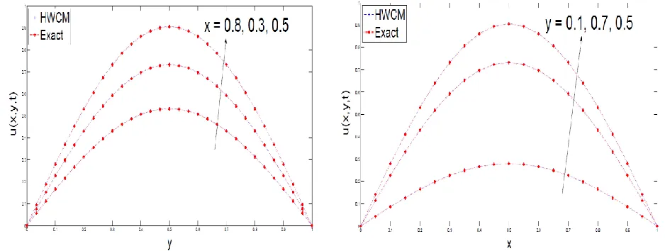
in Tables 1,2,3. The results are compared with the exact solution. Figures 1,2 show the comparison of the HWCM solution with the exact solution and the physical behavior of the
HWCM solution in contour and 3D at = 0.1t . If uex( , , )x y ts is the exact solution (28) at t=ts,
we define the error estimate as
1 2
1
( ) = ( , , ) ( , , )
2 2
s s ex s
t u x y t u x y t
M M
(29)
We have obtained the following error estimates for M1 = 16, M2 = 16 and t= 0.0001.
1. (0.01) = 5.2075E06 in L2 space and (0.01) = 6.6250E06 in L space.
2. (0.05) = 1.4590E05 in L2 space and (0.05) = 1.8561E05 in L space.
3. (0.1) = 1.5810E05 in L2 space and (0.1) = 2.0114E05 in L space.
Example 2:
2 2 2 2 2
1
= , 0 , 1, 0,
2
( , , 0) = 2 sin( ( )) sin( ( )), 0 , 1,
( , 0, ) = 0
0 1, 0,
( ,1, ) = 0
(0, , ) = 0
0 1, 0.
(1, , ) = 0
u u u
x y t
t x y
u x y x y x y x y
u x t
x t
u x t
u y t
y t
u y t
(30)
The exact solution is
1 1
( , , ) = cos cos
2 2
t
u x y t e x y
(31)
= 0.0001
t
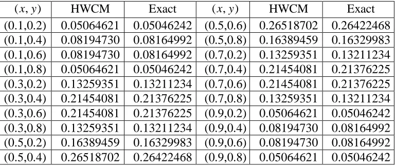
in Tables 4,5,6. The results are compared with the exact solution. Figures 3,4 show the comparison of the HWCM solution with the exact solution and the physical behavior of the
HWCM solution in contour and 3D at = 0.1t . We have obtained the following error estimates for
1= 16
M , M2 = 16 and t= 0.0001.
1. (0.01) = 2.9748E07 in L2 space and (0.01) = 3.7846E07 in L space.
2. (0.05) = 1.4352E06 in L2 space and (0.05) = 1.8259E06 in L space.
3. (0.1) = 7.2213E04 in L2 space and (0.1) = 9.1871E04 in L space.
Example 3:
2 2 2 2
1
= , 0 , 1, 0,
( , , 0) = (1 ) , 0 , 1
( , 0, ) =
0 1, 0,
( ,1, ) = 0
(0, , ) = (1 )
0 1, 0.
(1, , ) = (1 )
x
x t
t
t
u u u
x y t
t x y
u x y y e x y
u x t e
x t
u x t
u y t y e
y t
u y t y e
(32)
The exact solution is
( , , ) = (1 ) x t
u x y t y e (33)
The HWCM solution of the example at t = 0.01, 0.05, 0.1 with M1 = 4, M2 = 4 and t= 0.001
in Tables 7,8,9. The results are compared with the exact solution. Figures 5,6 show the comparison
of the HWCM solution with the exact solution and the physical behavior of the HWCM solution in
contour and 3D at = 0.1t . We have obtained the following error estimates for M1= 4, M2 = 4
and t= 0.001.
1. (0.01) = 1.8815E17 in L2 space and (0.01) = 3.0358E17 in L space.
2. (0.05) = 1.0148E16 in L2 space and (0.05) = 1.4615E16 in L space.
3. (0.1) = 1.0614E16 in L2 space and (0.1) = 1.2273E16 in L space.
6 Conclusion
In this paper, an efficient numerical scheme based on uniform Haar wavelets is used to solve
parabolic partial differential equation, namely, two-dimensional heat equation. The numerical
scheme is tested for three examples. The obtained numerical results are compared with the exact
solutions. We observe that the error estimates are negligibly small in the case of nonlocal boundary
guarantees the necessary accuracy with a small number of grid points and a wide class of PDEs can
be solved using this approach. This method takes care of boundary conditions automatically and
hence it is the most convenient method for solving boundary value problems. This method can also
Figure 1: Comparison of the HWCM solution and exact solution of Example 1 at = 0.1t
Figure 2: Physical behaviour of the HWCM solution of Example 1 at = 0.1t
[image:10.612.72.541.465.642.2]
Figure 4: Physical behaviour of the HWCM solution of Example 2 at = 0.1t
Figure 5: Comparison of the HWCM solution and exact solution of Example 3 at = 0.1t
Table 1: Comparison of HWCM solution and exact solution of Example 1 at = 0.01t
( , )x y HWCM Exact ( , )x y HWCM Exact (0.1,0.2) 0.29825855 0.29819802 (0.5,0.6) 1.56170205 1.56138509 (0.1,0.4) 0.48259247 0.48249453 (0.5,0.8) 0.96518495 0.96498905 (0.1,0.6) 0.48259247 0.48249453 (0.7,0.2) 0.78085103 0.78069254 (0.1,0.8) 0.29825855 0.29819802 (0.7,0.4) 1.26344350 1.26318707 (0.3,0.2) 0.78085103 0.78069254 (0.7,0.6) 1.26344350 1.26318707 (0.3,0.4) 1.26344350 1.26318707 (0.7,0.8) 0.78085103 0.78069254 (0.3,0.6) 1.26344350 1.26318707 (0.9,0.2) 0.29825855 0.29819802 (0.3,0.8) 0.78085103 0.78069254 (0.9,0.4) 0.48259247 0.48249453 (0.5,0.2) 0.96518495 0.96498905 (0.9,0.6) 0.48259247 0.48249453 (0.5,0.4) 1.56170205 1.56138509 (0.9,0.8) 0.29825855 0.29819802
Table 2: Comparison of HWCM solution and exact solution of Example 1 at = 0.05t
( , )x y HWCM Exact ( , )x y HWCM Exact (0.1,0.2) 0.13556365 0.13539405 (0.5,0.6) 0.70982048 0.70893244 (0.1,0.4) 0.21934659 0.21907217 (0.5,0.8) 0.43869318 0.43814434 (0.1,0.6) 0.21934659 0.21907217 (0.7,0.2) 0.35491024 0.35446622 (0.1,0.8) 0.13556365 0.13539405 (0.7,0.4) 0.57425683 0.57353839 (0.3,0.2) 0.35491024 0.35446622 (0.7,0.6) 0.57425683 0.57353839 (0.3,0.4) 0.57425683 0.57353839 (0.7,0.8) 0.35491024 0.35446622 (0.3,0.6) 0.57425683 0.57353839 (0.9,0.2) 0.13556365 0.13539405 (0.3,0.8) 0.35491024 0.35446622 (0.9,0.4) 0.21934659 0.21907217 (0.5,0.2) 0.43869318 0.43814434 (0.9,0.6) 0.21934659 0.21907217 (0.5,0.4) 0.70982048 0.70893244 (0.9,0.8) 0.13556365 0.13539405
[image:12.612.115.499.494.657.2]
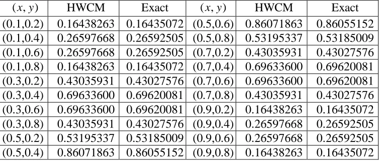
Table 3: Comparison of HWCM solution and exact solution of Example 1 at = 0.1t
( , )x y HWCM Exact ( , )x y HWCM Exact (0.1,0.2) 0.05064621 0.05046242 (0.5,0.6) 0.26518702 0.26422468 (0.1,0.4) 0.08194730 0.08164992 (0.5,0.8) 0.16389459 0.16329983 (0.1,0.6) 0.08194730 0.08164992 (0.7,0.2) 0.13259351 0.13211234 (0.1,0.8) 0.05064621 0.05046242 (0.7,0.4) 0.21454081 0.21376225 (0.3,0.2) 0.13259351 0.13211234 (0.7,0.6) 0.21454081 0.21376225 (0.3,0.4) 0.21454081 0.21376225 (0.7,0.8) 0.13259351 0.13211234 (0.3,0.6) 0.21454081 0.21376225 (0.9,0.2) 0.05064621 0.05046242 (0.3,0.8) 0.13259351 0.13211234 (0.9,0.4) 0.08194730 0.08164992 (0.5,0.2) 0.16389459 0.16329983 (0.9,0.6) 0.08194730 0.08164992 (0.5,0.4) 0.26518702 0.26422468 (0.9,0.8) 0.05064621 0.05046242
Table 4: Comparison of HWCM solution and exact solution of Example 2 at = 0.01t
( , )x y HWCM Exact ( , )x y HWCM Exact (0.1,0.2) 0.17983179 0.17982833 (0.5,0.6) 0.94161145 0.94159335 (0.1,0.4) 0.29097394 0.29096835 (0.5,0.8) 0.58194788 0.58193669 (0.1,0.6) 0.29097394 0.29096835 (0.7,0.2) 0.47080573 0.47079667 (0.1,0.8) 0.17983179 0.17982833 (0.7,0.4) 0.76177967 0.76176502 (0.3,0.2) 0.47080573 0.47079667 (0.7,0.6) 0.76177967 0.76176502 (0.3,0.4) 0.76177967 0.76176502 (0.7,0.8) 0.47080573 0.47079667 (0.3,0.6) 0.76177967 0.76176502 (0.9,0.2) 0.17983179 0.17982833 (0.3,0.8) 0.47080573 0.47079667 (0.9,0.4) 0.29097394 0.29096835 (0.5,0.2) 0.58194788 0.58193669 (0.9,0.6) 0.29097394 0.29096835 (0.5,0.4) 0.94161145 0.94159335 (0.9,0.8) 0.17983179 0.17982833
[image:13.612.121.495.278.443.2]
Table 5: Comparison of HWCM solution and exact solution of Example 2 at = 0.05t
( , )x y HWCM Exact ( , )x y HWCM Exact (0.1,0.2) 0.17279384 0.17277716 (0.5,0.6) 0.90476030 0.90467294 (0.1,0.4) 0.27958631 0.27955931 (0.5,0.8) 0.55917262 0.55911863 (0.1,0.6) 0.27958631 0.27955931 (0.7,0.2) 0.45238015 0.45233647 (0.1,0.8) 0.17279384 0.17277716 (0.7,0.4) 0.73196646 0.73189578 (0.3,0.2) 0.45238015 0.45233647 (0.7,0.6) 0.73196646 0.73189578 (0.3,0.4) 0.73196646 0.73189578 (0.7,0.8) 0.45238015 0.45233647 (0.3,0.6) 0.73196646 0.73189578 (0.9,0.2) 0.17279384 0.17277716 (0.3,0.8) 0.45238015 0.45233647 (0.9,0.4) 0.27958631 0.27955931 (0.5,0.2) 0.55917262 0.55911863 (0.9,0.6) 0.27958631 0.27955931 (0.5,0.4) 0.90476030 0.90467294 (0.9,0.8) 0.17279384 0.17277716
Table 6: Comparison of HWCM solution and exact solution of Example 2 at = 0.1t
( , )x y HWCM Exact ( , )x y HWCM Exact (0.1,0.2) 0.16438263 0.16435072 (0.5,0.6) 0.86071863 0.86055152 (0.1,0.4) 0.26597668 0.26592505 (0.5,0.8) 0.53195337 0.53185009 (0.1,0.6) 0.26597668 0.26592505 (0.7,0.2) 0.43035931 0.43027576 (0.1,0.8) 0.16438263 0.16435072 (0.7,0.4) 0.69633600 0.69620081 (0.3,0.2) 0.43035931 0.43027576 (0.7,0.6) 0.69633600 0.69620081 (0.3,0.4) 0.69633600 0.69620081 (0.7,0.8) 0.43035931 0.43027576 (0.3,0.6) 0.69633600 0.69620081 (0.9,0.2) 0.16438263 0.16435072 (0.3,0.8) 0.43035931 0.43027576 (0.9,0.4) 0.26597668 0.26592505 (0.5,0.2) 0.53195337 0.53185009 (0.9,0.6) 0.26597668 0.26592505 (0.5,0.4) 0.86071863 0.86055152 (0.9,0.8) 0.16438263 0.16435072
[image:13.612.119.496.495.658.2]Table 7: Comparison of HWCM solution and exact solution of Example 3 at = 0.01t
( , )x y HWCM Exact ( , )x y HWCM Exact (0.1,0.2) 0.89302246 0.89302246 (0.5,0.6) 0.66611648 0.66611648 (0.1,0.4) 0.66976684 0.66976684 (0.5,0.8) 0.33305824 0.33305824 (0.1,0.6) 0.44651123 0.44651123 (0.7,0.2) 1.62719301 1.62719301 (0.1,0.8) 0.22325561 0.22325561 (0.7,0.4) 1.22039476 1.22039476 (0.3,0.2) 1.09074009 1.09074009 (0.7,0.6) 0.81359650 0.81359650 (0.3,0.4) 0.81805507 0.81805507 (0.7,0.8) 0.40679825 0.40679825 (0.3,0.6) 0.54537005 0.54537005 (0.9,0.2) 1.98745803 1.98745803 (0.3,0.8) 0.27268502 0.27268502 (0.9,0.4) 1.49059352 1.49059352 (0.5,0.2) 1.33223296 1.33223296 (0.9,0.6) 0.99372901 0.99372901 (0.5,0.4) 0.99917472 0.99917472 (0.9,0.8) 0.49686451 0.49686451
[image:14.612.122.495.278.442.2]
Table 8: Comparison of HWCM solution and exact solution of Example 3 at = 0.05t
( , )x y HWCM Exact ( , )x y HWCM Exact (0.1,0.2) 0.92946740 0.92946739 (0.5,0.6) 0.69330121 0.69330121 (0.1,0.4) 0.69710055 0.69710055 (0.5,0.8) 0.34665060 0.34665060 (0.1,0.6) 0.46473370 0.46473370 (0.7,0.2) 1.69360001 1.69360001 (0.1,0.8) 0.23236685 0.23236685 (0.7,0.4) 1.27020001 1.27020001 (0.3,0.2) 1.13525404 1.13525404 (0.7,0.6) 0.84680001 0.84680001 (0.3,0.4) 0.85144053 0.85144053 (0.7,0.8) 0.42340000 0.42340000 (0.3,0.6) 0.56762702 0.56762702 (0.9,0.2) 2.06856773 2.06856773 (0.3,0.8) 0.28381351 0.28381351 (0.9,0.4) 1.55142580 1.55142580 (0.5,0.2) 1.38660241 1.38660241 (0.9,0.6) 1.03428386 1.03428386 (0.5,0.4) 1.03995181 1.03995181 (0.9,0.8) 0.51714193 0.51714193
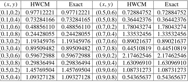
Table 9: Comparison of HWCM solution and exact solution of Example 3 at = 0.1t
( , )x y HWCM Exact ( , )x y HWCM Exact (0.1,0.2) 0.97712221 0.97712221 (0.5,0.6) 0.72884752 0.72884752 (0.1,0.4) 0.73284166 0.73284165 (0.5,0.8) 0.36442376 0.36442376 (0.1,0.6) 0.48856110 0.48856110 (0.7,0.2) 1.78043274 1.78043274 (0.1,0.8) 0.24428055 0.24428055 (0.7,0.4) 1.33532456 1.33532456 (0.3,0.2) 1.19345976 1.19345976 (0.7,0.6) 0.89021637 0.89021637 (0.3,0.4) 0.89509482 0.89509482 (0.7,0.8) 0.44510819 0.44510819 (0.3,0.6) 0.59672988 0.59672988 (0.9,0.2) 2.17462546 2.17462546 (0.3,0.8) 0.29836494 0.29836494 (0.9,0.4) 1.63096910 1.63096910 (0.5,0.2) 1.45769504 1.45769504 (0.9,0.6) 1.08731273 1.08731273 (0.5,0.4) 1.09327128 1.09327128 (0.9,0.8) 0.54365637 0.54365637
[image:14.612.123.494.494.657.2]Acknowledgements
The authors are obliged to Prof. N. M. Bujurke, INSA Senior Scientist for introducing them to
Haar wavelets and providing needful inputs during the preparation of this manuscript. The first
author is thankful to the University Grants Commission (UGC) for their financial support through
Award No.: MRP(S)-0385/13-14/KABA031/UGC-SWRO, Bangalore. The third author is
thankful to Vision Group of Science and Technology (VGST) for providing financial assistance
through GRD 105, CISE.
References
[1] T. Myint-U, L. Debnath, Linear partial differential equations for scientists and engineers, Birkhauser, 2011.
[2] K. Tabatabaei, E. Celik, R. Tabatabaei, The differential transform method for solving
heat-like and wave-like equations with variable coefficients, Turk. J. Phys. 36 (2012) 87-98.
[3] X.G. Luo, Q.B. Wu, B.Q. Zhang, Revisit on partial solutions in the Adomian decomposition method: Solving heat and wave equations, J. Math. Anal. Appl. 321(1) (2006) 353-363.
[4] A. Cheniguel, A. Ayadi, Solving heat equation by the Adomian decomposition method, Proc. World Cong. Engg. 1 (2011).
[5] M. Mahalakshmi, R. Rajaraman, G. Hariharan, K. Kannan, Approximate analytical solutions of two dimensional transient heat conduction equations, Appl. Math. Sci. 6(71) (2012) 3507-3518.
[6] J. Douglas Jr., D.W. Peaceman, Numerical solution of two-dimensional heat-flow problems, Amer. Inst. Chem. Engg. 1(5) (1955) 505-512.
[7] C.N. Dawson, Q. Du, T.F. Dupont, A finite difference domain decomposition algorithm for numerical solution of the heat equation, Math. Comput. 57(195) (1991) 63-71.
[8] J.C. Bruch Jr., G. Zyvoloski, Transient two-dimensional heat conduction problems solved by the finite element method, Int. J. Num. Methods Engg. 8(3) (1974) 481-494.
[9] S. Adjerid, J.E. Flaherty, A moving-mesh finite element method with local refinement for parabolic partial differential equations, Comp. Methods Appl. Mech. Engg. 55(1-2) (1986) 3-26.
[11] J.S. Hicks, J. Wei, Numerical solution of parabolic partial differential equations with two-point boundary conditions by use of the method of lines, J. ACM 14(3) (1967) 549-562.
[12] J. Villadsen, J.P. Sorensen, Solution of parabolic partial differential equations by a double collocation method, Chem. Engg. Sci. 24(8) (1969) 1337-1349.
[13] M. Tatari, M. Dehghan, On the solution of the non-local parabolic partial differential equations via radial basis functions, Appl. Math. Model. 33(3) (2009) 1729-1738.
[14] M. Siddique, Numerical computation of two-dimensional diffusion equation with nonlocal boundary conditions, Int. J. Appl. Math. 40(1) (2010).
[15] R.S. Sumana, L.N. Achala, A short report on different wavelets and their structures, Int. J. Res. Engg. Sci. 4(2) (2016) 31-35.
[16] U. Lepik, Numerical solution of differential equations using Haar wavelets, Math. Comput. Simul. 68 (2005) 127-143.
[17] M. Khalid, M. Sultana, F. Zaidi , Numerical solution of Airy differential equation by using Haar wavelet, Math. Th. Model. 4(10) (2014) 142-148.
[18] Z. Shi, Y. Cao, Application of Haar wavelet method to eigenvalue problems of high order differential equations, Appl. Math. Model. 9 (2012) 4020-4026.
[19] U. Lepik, Numerical solution of evolution equations by the Haar wavelet method, Appl. Math. Comput. 185 (2007) 695-704.
[20] N. Bujurke, C. Salimath, R. Kudenatti, S. Shiralashetti, A fast wavelet-multigrid method to solve elliptic partial differential equations, Appl. Math. Comput. 185 (2007) 667-680.
[21] U. Lepik, Solving PDEs with the aid of two-dimensional Haar wavelets, Comput. Math. Appl. 61 (2011) 1873-1879.