2017 International Conference on Mathematics, Modelling and Simulation Technologies and Applications (MMSTA 2017) ISBN: 978-1-60595-530-8
Parametric Acoustic Receiving Array in Two-phase Media
Song-wen LI
Shanghai Marine Electronic Equipment Research Institute
Key Laboratory on Science and Technology of Underwater Acoustic Antagonizing, #5200 Jindu Road, 201108, Shanghai, China
Keywords: Parametric acoustic receiving array, Two-phase media, Slow acoustic velocity medium.
Abstract. Parametric acoustic receiving array can achieve higher space gain with relatively small (virtual) array aperture compare with ordinary line array. The amplitude of the secondary signals of parametric receiving array is proportional to the third power of the acoustic velocity of the medium, and two-phase media is much more practical than single medium with slow acoustic velocity in underwater acoustic engineering. Two-phase media model and equations for the secondary signals of parametric acoustic array are proposed and some calculation examples are given and analyzed.
Introduction
Parametric acoustic receiving array exploits nonlinear acoustic effects in fluids to form virtual end-fire array to realize directive reception of low frequency acoustic signal [1]. It needs only a pair of
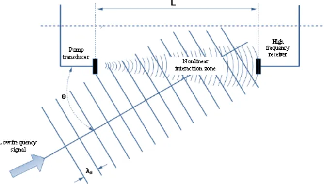
[image:1.612.141.475.400.590.2]transmitting-receiving high frequency acoustic transducers to form a parametric receiving array to achieve directive reception of low frequency signal, and is suitable for some kind of applications in underwater acoustic engineering where the space for the apparatus is limited in some way.
Figure 1. Diagram of parametric acoustic receiving array.
Fig. 1 shows the principle of parametric receiving array: a strong high frequency signal (called
pump signal, with frequency f0) projected from the pump transducer meets the weak low frequency
signal (signal to be detected, with frequency fs) in the nonlinear interaction zone. On account of the
received by the high frequency receiver are accumulated through the length L and have the property of an end-fire array with length L, which is directional. The low frequency signal to be detected can be resumed by demodulation of the secondary signal.
The amplitude of the secondary signals of parametric receiving array is proportional to the third power of the acoustic velocity of the medium [2]. If the acoustic velocity of the medium is much
slower than that of the water, much larger secondary signals can be obtain and make it easier to be detected in underwater acoustic engineering [3]. Usually the length of parametric acoustic receiving
array is as long as more than 100m in order to get large space gain, this makes it more suitable to use medium of slow acoustic velocity only in part of the whole length, and with the remain part still water. That means the parametric receiving array is in two-phase media. There is no suitable model for the prediction of the property of parametric receiving array in two-phase media right now.
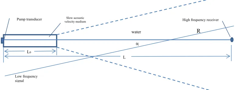
[image:2.612.113.502.252.400.2]Model and Equations
Figure 2. Diagram of two-phase medium parametric acoustic receiving array.
Fig. 2 is the diagram of a two-phase media parametric receiving array. The slow acoustic velocity
medium is on the side of the pump transducer, expanding from the pump transducer to L0 along the
pump wave axis. L0 is smaller than Reighly distance and the pump wave can be considered as plane
wave in this medium. The pump wave is spherical wave in water as normal parametric acoustic array
[2]. Then, the total secondary signal received by the high frequency receiver is combined by two parts:
those generated in the slow acoustic velocity medium traveled to the receiver and the those generated in water traveled to the receiver.
There are two kinds of virtual source: q0 in water and q1 in the slower acoustic velocity medium.
The low frequency signal is assumed to be plane wave signal, and only signals on the pump wave axis need to be considered [2], from the equation (3) in reference [2] we have
) /(
) (
0 )
' ( ' 2 1 4 0 2 0
2 1 0
2 1 0 1
0 r L
e P P c A
q L r jk L kr kR
r > L0 (1)
) ' ' ( ' 2 1 4 0 2 0
2 1 1
2 1
' ' ' '
)
( r jk r k R
e P P c
q
r ≤ L0 (2)
Here ω1 andω2 is the angular frequency of pump and low frequency signal, respectively. ρ0, c0, ρ’0,
c’0 is the density and acoustic velocity in water, and the density and acoustic velocity in the slow
acoustic velocity medium, respectively. α, α’ is the absorption coefficient in water and in the slow acoustic velocity medium, respectively. k1, k2, k’1, k’2 is the wave number of pump and low
frequency signal in water, and the wave number of pump and low frequency signal in the slow
Pump transducer velocity medium Slow acoustic High frequency receiver
water R
Low frequency signal
θ(
and A is the transmission loss when the pump wave traveling from slow acoustic velocity medium to water.
a) Secondary signal generated by the virtual sources in the slow acoustic velocity medium.
P’1 is the amplitude of the pump wave on the surface of a piston pump source. When there is no
slow acoustic velocity medium adhere to the transducer, the amplitude on the surface is Ps=P0λ1/S.
Considering the acoustic power projected is constant, and
0 0 2 1 0 0 2 ' ' ' c P c P E s (3) E is the acoustic power, Then
0 0 0 0 1 0 1 ' ' ) / ( ' c c S P P (4) P2 and P’2 is the amplitude of the low frequency signal in water and in the slow acoustic velocity
medium, respectively. For plane pump wave, the particle velocity at point (r, 0)is
r q
u
1 (5) From point (L0, 0) the pump signal will be expanding spherically, and the amplitude of the
secondary signals generated by the virtual source in the slow acoustic velocity medium will reduced to 1 / (L - L0) of the original when travelling to the point (L, 0). The acoustic absorption and the phase
change of the signals should be considered separately in these two media. Then
)) ( ) ( ' ( ) ( ) ( ' ( 0 0 0 0
0 r L L j k L r k L L
L
L L L e
u A
u
(6) Here A is the transmission loss of the sum frequency signal (the sum frequency is very close to the pump wave frequency, this loss is almost no difference), and k+ and k’+ is the wave number of sum
frequency signal in water and in the slow acoustic velocity medium respectively. Only sum frequency is considered here because the principle for the difference frequency signal is the same. Then, the contribution of the sum frequency signal at the point of receiver from the virtual sources in the slow acoustic velocity medium is
dr e e P P L L c A dr e P P L L c A c dr e L L q A c U c P L r jk L k L k L k j L L L L L L k r L k j L L r L R k r k j r L L L k r L k j L L r L L n
0 2 0 0 0 0 0 0 0 0 0 2 1 0 0 0 0 0 0 ) cos 1 ( ' ) ' ( ) ( ' 2 1 0 3 0 0 2 1 0 )) ( ) ( ' ( ) ( ) ( ' ) ' ' ( ' 2 1 0 4 0 2 0 2 1 0 0 0 )) ( ) ( ' ( ) ( ) ( ' ( 0 1 0 0 0 0 ' ' ) )( ' ' ( ) ( ' ' ) )( ' ' ( ) ( ' ' ' ' ' ' (7)b) Secondary signal generated by the virtual sources in water
Since the pump wave in water is spherical wave, the particle velocity at point (r, 0) when r>L0 is:
r q
u
0
2 1 '
(8) The signals generated by the virtual sources in water are expanded spherically. The expanding radium at point (r, 0) when r > L0 is r - L0 while the expanding radium at point (L, 0) is L - L0, then the
amplitude of the signal generated at point (r, 0) will reduced to (r-L0) / (L-L0) of the original when
)) ( ) ( ( 0 0) '
(
' L r jk L r
L e L L u L r A
u
(9)
The contribution of the sum frequency signal at the receiver from the virtual sources in water is
L L r jk L jk L L jk L L L r L jk r L R k r k L k j r L L L r L jk r L L f dr e e P P L L c A dr e P P L L c A c dr e L L q L r c U c P 0 2 0 1 0 0 2 1 0 1 0 0 ) cos 1 ( ' ' 2 1 0 3 0 0 2 1 ) ( ) ( ) ' ( ' 2 1 0 4 0 2 0 2 1 0 0 ) ( ) ( 0 0 ) 0 0 0 0 0 ) ( ) ( ) ( ) ( ) ( ' (10)Finally, the sum frequency signal generated by the parametric receiving array shown in fig. 2 will be
Pd = Pn + Pf (11)
Calculation Example
Rubber with density 0.1, acoustic velocity 1000m/S, absorption coefficient 1dB/m at frequency 100 kHz and nonlinear coefficient 4.97, is chosen for the calculation. Although the acoustic velocity in rubber is much slower than that in water, it is not proper to choose a very large L0. The strong power
absorption of the rubber may cause the increased absorption effects greater than the increased nonlinear effects if L0 is too large, and the secondary signal may decrease instead of increase. Except
the secondary signal is still high enough even if L0 is very large, and the ratio of the pump signal and
the secondary signal may decrease because of the higher nonlinear transmission efficiency in rubber to make it easier to extract the weak secondary signals from the jam caused by the strong pump signal. The transmission loss for the secondary signal traveling from rubber to water is
75 . 0 ) ' ' /( ' ' 2
1 0c 0 0c 0 0c0
t
The pump source level is chosen to be 230dB re. 1uPa and aperture is 450x225mm2. For the pump frequency of 100 kHz, Ps=213dB, P1’=211dB, and Reighly distance is 6.7m. Sound level of the low frequency signal is 40dB and frequency is 2 kHz. L0=5m (0.75 Reighly distance).
Table 1 shows the comparison between parametric receiving array in water and in rubber-water two-phase media.
Table 1. Comparison between parametric acoustic receiving array in water and in rubber-water two-phase media.
L0 (m) L(m)
Sound level of sum frequency signal (dB)
Ratio of pump and sum frequency signal (dB)
In water In two-phase
media In water
In two-phase media
5
5 23 31 185 175
10 26 24 189 183
20 26 20 180 179
100 26 18.5 165 165
Reference
[1] H.O. Berktay, Parametric amplification by the use of acoustic nonlinearities and some possible applications, J, Sound Vib., 462-470, 2, 1965.
[2] H.O. Berktay and J.A. Shooter, Parametric receiver with spherically spreading pump waves, J. Acoust. Soc. Am, 1056-1061, 54(4), 1973.
[3] R.D. Corsaro and J. Jarzynski, “Compact parametric hydrophone using nonlinear interaction within a cylindrical rubber waveguide, J. Acoust. Soc. Am, 895-904, 66(3), 1979.
[4] H.O. Berktay and T.G. Muir, Arrays of parametric receiving arrays, J. Acoust. Soc. Am, 1377-1383, 53(5), 1973.