DOI: 10.1111/phor.12259
GPS PRECISE POINT POSITIONING FOR UAV
PHOTOGRAMMETRY
Ben GRAYSON*([email protected]) Nigel T. PENNA([email protected])
Jon P. MILLS([email protected])
Newcastle University, Newcastle upon Tyne, United Kingdom
Darion S. GRANT([email protected])
University of East London, London, United Kingdom
*Corresponding author
Abstract
The use of Global Positioning System (GPS) precise point positioning (PPP) on a fixed-wing unmanned aerial vehicle (UAV) is demonstrated for photogrammetric mapping at accuracies of centimetres in planimetry and about a decimetre in height, fromflights of 25 to 30 minutes in duration. The GPS PPP estimated camera station positions are used to constrain estimates of image positions in the photogrammetric bundle block adjustment, as with relative GPS positioning. GPS PPP alleviates all spatial operating constraints associated with the installation and the use of ground control points, a local ground GPS reference station or the need to operate within
the bounds of a permanent GPS reference station network. This simplifies
operational logistics and enables large-scale photogrammetric mapping from UAVs in even the most remote and challenging geographic locations.
Keywords:direct georeferencing, GPS, precise point positioning, structure from motion, unmanned aerial vehicle
Introduction
UNMANNED AERIAL VEHICLES (UAVs) have recently become a popular platform for photogrammetric data acquisition because of their flexible nature and low cost in comparison to manned aerial platforms (Colomina and Molina, 2014). Moreover, products such as dense point clouds, digital elevation models and orthomosaics are now routinely obtainable from UAV imagery with centimetre-level accuracy using only a small number of high-accuracy ground control points (GCPs) (for example, Lucieer et al., 2014; Peppa et al., 2016; Reshetyuk and Martensson, 2016; Murtiyoso and Grussenmeyer, 2017). Such GCPs have traditionally been required for the indirect determination of absolute image orientations during aerial triangulation, as typically implemented through a bundle block adjustment. However, establishing well-distributed GCPs is a time-consuming, costly and often difficult
process to implement, especially in mountainous terrain (Micheletti et al., 2015) or glaciated areas (Immerzeel et al., 2014; Kraaijenbrink et al., 2016). Eliminating the requirement for GCPs is therefore highly desirable.
For conventional photogrammetry using manned aerial platforms, Heipke et al. (2002) showed that GCPs may be removed by making direct measurements of absolute camera positions and attitudes using an onboard Global Positioning System (GPS) receiver, antenna and inertial measurement unit (IMU). These may be held fixed for the extrapolation of mapping coordinates using direct sensor orientation (Yastikli and Jacobsen, 2005) or, alternatively, used to constrain image orientation estimates in a bundle block adjustment in the integrated sensor orientation approach (Cramer et al., 2000; Ip et al., 2007). Integrated sensor orientation offers improvements in mapping accuracy and reliability over direct sensor orientation because the inclusion of image tie points allows a refinement of relative orientation (by reducing y-parallax error), as offered by aerial triangulation (Heipke et al., 2002). Image tie points also enable the estimation of camera attitudes and thus they can eliminate the need for IMU observations in so-called GPS-supported aerial triangulation, provided a block geometry of several overlapping strips exists (Ackermann and Schade, 1993). However, without GCPs, these approaches remain susceptible to mapping errors incurred by prevalent systematic error or “drifts” in GPS camera positions. Thus, to date, conventional aerial photogrammetry typically involves reducing GCPs to a minimal number of four points, one located in each corner of the image block. This configuration has been demonstrated to enable the accurate estimation, or elimination, of these errors, preventing their propagation into final mapping coordinates (Ackermann and Schade, 1993; Ackermann, 1994; Ip et al., 2007; Yuan, 2009; Shi et al., 2017). (Note that although the
Recordgenerally adopts the generic Global Navigation Satellite System (GNSS), this paper follows the geodetic convention of using GPS where observations solely from that system are used, as is the case here.)
Photogrammetry from UAV platforms, unlike manned aerial platforms, usually necessitates the use of structure from motion (SfM) techniques to facilitate the bundle block adjustment (for example, Harwin and Lucieer, 2012; Peppa et al., 2016). This is because SfM provides efficient and direct solutions (so no requirement for a priori information) to the matching and relative orientation of convergent and non-metric small-format imagery. Control information (such as GCPs or camera positions) may then be integrated as additional parameter observations in a rigorous bundle block adjustment, thus conforming to aerial triangulation. The latter step may also be satisfied by a Helmert (three-dimensional conformal) transformation, but this has limited accuracy because the control information does not help to minimise possible block deformations and systematic errors (James and Robson, 2012; Nex and Remondino, 2014).
A major factor influencing the accuracy of UAV point clouds derived using direct georeferencing (thus in the absence of GCPs) is the quality of GPS-based camera positions. Amongst other factors such as block geometry, image measurement quality and ground sample distance (GSD), GPS positions accurate to the centimetre level can assist in yielding mapping also with centimetre accuracy (Turner et al., 2014). Code-based GPS positioning techniques are of limited value in large-scale mapping applications if GCPs are to be completely removed (Turner et al., 2012). For example, stand-alone single frequency pseudorange GPS positioning has a positional accuracy of approximately 5 to 10 m, while differential pseudorange GPS (DGPS) techniques, which became popular in the 1990s, provide typical accuracies of around 05 to 1 m (Chen et al., 2009). To obtain GPS-based camera positions with centimetre-level accuracy, dual-frequency carrier phase and code observations are therefore required. If a local GPS reference (base) station is available, relative GPS positioning in the form of post-processed kinematic (PPK) GPS or, with a radio link, real-time kinematic (RTK) GPS may be used. In relative positioning, GPS carrier phase observations are double differenced to solve for positions relative to the (known) reference station coordinates. If the baselines are short (less than a few kilometres) and the double differenced ambiguities are successfully resolved to integers, then PPK/RTK GPS positions with centimetre accuracy can result (Han, 1997). A third form of relative carrier phase GPS positioning that may be adopted is network RTK, for example, using the virtual reference station method (for example, Hu et al., 2003), which involves corrections being sent to the user from a network of GPS reference stations. However, the area being surveyed must fall within the bounds of such a network, which often only prevail in urban areas in developed countries, whilst also requiring a subscription to a suitable network RTK service.
The GPS precise point positioning (PPP) technique (Zumberge et al., 1997) provides a potential alternative to relative GPS for the determination of camera station positions with centimetre-level precision and accuracy. Instead of differencing observations with respect to a known ground-based GPS reference station, the PPP technique involves the fixing of highly accurate satellite orbit and clock parameters such as those that have long been freely available through the International GNSS Service (IGS) (Heroux and Kouba, 2001). A stand-alone position is then estimated directly, using dual-frequency carrier phase and code GPS data, and the PPP technique has been extended from static to kinematic modes through the availability of accurate high-rate (such as 5- to 30-second rather than 5-minute) satellite clocks. The main drawback of the approach is that integer ambiguity resolution is not possible in pure stand-alone PPP mode without additional data from reference stations, as ambiguities are contaminated by hardware delays (Bertiger et al., 2010). Ambiguities must therefore be estimated as float values. Reliable estimation requires their separation from other estimated parameters (tropospheric delay, receiver clock and coordinates), which depends on the satellite geometry changing sufficiently such that non-singular normal equations arise in the least squares estimation, usually requiring at least 15 to 20 minutes of observation. However, with accurate float-ambiguity estimation, centimetre-level accuracy positioning becomes possible. For example, Cai and Gao (2013) and Yu and Gao (2017) obtained centimetre-level horizontal accuracies from land-based vehicle tests, although the heighting accuracy found by Cai and Gao (2013) was nearly a decimetre.
also makes accurate GPS positioning more challenging. Gross et al. (2016) undertook kinematic PPP on three UAV missions, but with flight durations in the range of 26 to 57 minutes. These resulted in reported UAV positioning accuracies in the range of 061 to 139 m, albeit with centimetre-level precision. The low accuracy was attributed to the estimated float ambiguities not converging to their true values, and hence such results cannot be used for direct georeferencing in large-scale photogrammetric mapping applications without the use of GCPs. Yuan et al. (2009) used PPP for GPS-supported aerial triangulation on manned aerial platforms with flight durations exceeding 5 hours. For a project comprising 1:2500 scale imagery, with nine strips and two cross strips (scanned with a resolution of 21lm), PPP and relative GPS baseline trajectories agreed to within approximately 80, 50 and 120 cm in easting, northing and height, respectively, although the agreements degraded during the flight due to worsening satellite geometries. Because of these PPP biases, four GCPs were included in the GPS-supported bundle block adjustment and used to solve for systematic error parameters on a strip-by-strip basis. Root mean square errors (RMSEs) of better than 15 cm were then reported at independent check points on the ground. This work was extended to real-time PPP using predicted satellite orbits by Shi et al. (2017), again using a manned aerial platform with a flight duration exceeding 4 hours. For a project comprising 15 strips, differences of up to 50 cm were reported between real-time and post-processed PPP camera positions, but these were compensated in the bundle block adjustment usingfive GCPs, as with Yuan et al. (2009), to achieve check point RMSEs of 10 to 20 cm for all solutions.
To date, the application of GPS PPP for direct georeferencing in airborne mapping has resulted in low accuracy on small UAV platforms, or has been utilised on manned aerial platforms with flight durations of several hours and incorporating GCPs to compensate for GPS PPP biases. This paper investigates whether direct georeferencing of a lightweight,
fixed-wing UAV platform for use in large-scale mapping is possible by using kinematic GPS PPP. It seeks to eliminate the need for GCPs, a local GPS reference station orflying within the bounds of a network RTK GPS correction network. The UAV GPS PPP positions are first assessed by comparison with GPS PPK solutions. Following this, the accuracy and precision of mapping obtained by GPS PPP direct georeferencing is assessed through independent check point errors, which are directly compared with those obtained from an indirect approach using a GCP-based bundle block adjustment.
Data Acquisition
Test Field and UAV Missions
GNSS receiver. The flying height above ground level in both missions was approximately 120 m, which resulted in an image GSD of approximately 3 cm. Ground targets thus appeared in the obtained imagery as about 9 pixels in diameter, with the inner spot appearing as about 3 pixels. The camera was triggered every 2 seconds during the flights, with precise camera exposure events fed into the Q-200’s data logger from the camera hot-shoe attachment. This enabled the recording of camera exposure times with an expected accuracy of 5 to 10 ms (Rehak and Skaloud, 2017b) for synchronisation with the GPS observations. Dual-frequency (L1/L2) carrier phase and code GPS observations were logged at 10 Hz throughout both missions. The survey details are summarised in Table I.
The flight plan for both missions consisted of 16 strips running east–west, with two cross strips running north–south, although the second cross strip was not obtained for Flight 1 due to battery exhaustion. As with many such small UAV systems, the Q-200’s batteries limit flight durations to a maximum of 20 to 30 minutes, which is further influenced by local wind speeds and temperature. To maximise flight durations, necessary to improve the estimation of GPS PPP ambiguities, the Q-200 was manually piloted after completion of the automated flight plan and not landed until battery voltage readings dropped to a critical level. This resulted in launch-to-landing durations for Flights 1 and 2 of 25 and 29 minutes, respectively.
Ground Survey
[image:5.485.58.427.74.307.2]To coordinate the ground targets (GCPs and check points), a local GPS reference station (Leica GS10 receiver with AS10 antenna) was established in the central grass field
Fig. 1. Testfield at Cockle Park, Northumberland, north-east England. Flight lines (for Flight 1 only), location
(Fig. 1), logging at 5 Hz from 09:12 to 13:36 UTC on 15th August 2017 and then from 07:01 to 15:08 UTC on 16th August 2017. The ground targets were coordinated twice, once pre-flight on 15th August and again, as a check, post-flight on 16th August. All ground targets were occupied for 3 minutes per survey with a roving Leica GS10 receiver and AS10 antenna, using“static + kinematic” mode over the course of approximately 3 hours on each day. Adopting this survey mode meant that the rover continuously logged data for up to 3 hours, enabling a continuous, long GPS data arc to ensure reliable integer ambiguity resolution. The rover data were processed relative to thefixed coordinates of the local GPS reference station using Leica Infinity version 2.1.0 software, with the processing parameters listed in Table II. Baseline lengths were very short, at no more than 300 m. The 3D RMSE coordinate difference for the 40 ground targets between the two surveys was 12 mm.
[image:6.485.74.417.80.233.2]As the coordinate reference frame for GPS PPP direct georeferencing is defined by the frame of the fixed satellite orbits (here IGS14: the IGS realisation of the International Terrestrial Reference Frame 2014 at the epoch of date), it was critical for comparison purposes to also coordinate the ground targets in the same frame. Noting that the frame of the ground targets is defined according to the fixed coordinates of the local GPS reference station, this needed to be coordinated using the same GPS PPP processing as used for the UAV processing (details described below and in Table II). However, only 8 hours of data
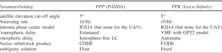
Table II.GPS processing parameters.
Parameter/setting PPP (PANDA) PPK (Leica Infinity)
Satellite elevation cut-off angle 5° 5°
Processing rate 10 Hz 10 Hz
Antenna phase centre model IGS14 (but none for the UAV) IGS14 (but none for the UAV) Tropospheric delay Estimated VMF with GPT2 model Ionospheric delay Ionosphere-free LC Automatic
Precise orbit/clock product CODE CODE
Ambiguity solution Float Fixed
[image:6.485.66.428.498.585.2]VMF = Vienna Mapping Function; GPT2 = Global Pressure and Temperature model (Lagler et al., 2013); CODE=Centre for Orbit Determination in Europe.
Table I.Survey details.
Specification Details
UAV aircraft/system Quest Q-200
Date of image acquisition 16th August 2017
Camera Sony DSC-ILCE-6000
Nominal focal length 16 mm
Flying height 120 m
Flight 1 timings 09:25 to 09:50 UTC (25 min)
Flight 2 timings 10:44 to 11:13 UTC (29 min)
No. of images (Flight 1, Flight 2) 406, 473
GSD 30 mm
GCPs (when used) 16
Check points 24
were collected at the local GPS reference station and, as GPS satellite geometry varies over the course of a sidereal day (approximately 23 hours 56 minutes), there was a potential for the computed local GPS reference station coordinates to be biased by the time-of-day satellite geometry, as the accuracy of PPP solutions are particularly sensitive to geometric effects (for example, Marques et al., 2018). To overcome this, the 8 hours of observed reference station GPS data were processed with Leica Infinity relative to reference station MORP (Morpeth, Northumberland, north-east England), one of about 500 continuously operating reference stations operated by IGS and conveniently located only 600 m away. The coordinates of MORP were themselves determined by averaging kinematic GPS PPP positions processed by the same method as used for the UAV (see below, and hence in the same IGS14 reference frame defined by the satellite orbits). However, 48 hours of data were used to ensure averaging out of sidereal day repeat geometric variations and estimating a constant zenith wet tropospheric delay per hour. Thus, the local reference station was coordinated in the frame of the satellite orbits, and using the same kinematic processing method as for the UAV (rather than the conventional static approach) ensured complete compatibility with the UAV GPS kinematic PPP positions for evaluation purposes.
GPS Analysis
UAV Reference Trajectory
To assess the accuracy of the GPS PPP positions on the UAV, a reference trajectory was computed by processing the GPS data from the two missions in GPS PPK mode, relative to the local GPS reference station. Leica Infinity with the processing settings listed in Table II was used, with the same reference station coordinates fixed as for the coordination of the ground targets. Ambiguities were successfully fixed to integers for all epochs of both missions. The assumed precision and accuracy of this trajectory was 2 to 3 cm. It should be noted that the local GPS reference station only logged at 5 Hz, while the UAV logged at 10 Hz and Leica Infinity output positions at the 10 Hz UAV rate. However, to ensure compatibility with the GPS reference station observation sampling rate, only 5 Hz PPK positions were used as truth to assess the accuracy of the PPP estimated positions.
GPS PPP Processing Method
trajectory. This aspect is important from a photogrammetric viewpoint, as it enables the determination of camera positions with a homogenous accuracy so that all such observations may be weighted equally in the bundle block adjustment.
Satellite orbit and 5-second clocks were obtained from the Centre for Orbit Determination in Europe (CODE) IGS Analysis Centre, which were thenfixed in the least squares estimation, and the GPS data were processed at a rate of 10 Hz. Five-second clocks were used rather than the 30-second clocks provided in the final combined IGS product because Bock et al. (2009) showed that satellite clock interpolation (and subsequent positioning) errors can be reduced by using clocks provided at 5 rather than 30 seconds. The PANDA processing parameters provided in Table II were used in all GPS PPP solutions unless otherwise specified hereafter. Unfortunately, an antenna phase centre variation model (whose application improves mainly the height component, as detailed in Mader, 1999) was not available for the UAV’s Maxtena antenna and so corrections were not applied for the UAV antenna. For further details on GPS PPP processing, see Kouba and Heroux (2001).
Quality Assessment of GPS PPP UAV Trajectories
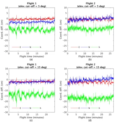
The determined GPS PPP coordinate errors, defined as the differences between the PPP and PPK reference trajectory coordinates, for each 5 Hz epoch (matching the GPS reference station sampling rate) for the full durations of Flights 1 and 2 are displayed in Fig. 2. They are shown for processing using satellite elevation cut-off angles of both 5° and 15°. The mean error and standard deviation error statistics for the 5°elevation cut-off angle processing are listed in Table III. Fig. 2 shows that the planimetric coordinate errors remain below 5 cm for bothflights, with the satellite elevation cut-off angle having minimal effect. As can be seen from Table III, the mean error for any of the planimetric coordinates for the 5°cut-off case is at most 33 cm. However, height errors in Fig. 2 are greater, with mean errors of 102 and 92 cm for Flights 1 and 2, respectively. Larger height than planimetric errors are expected because of the inherent satellite geometric distribution (with any range errors directly propagating to the estimated heights), whereas precisions (standard deviations) of better than 2 cm are obtained for all coordinate components. When increasing the satellite elevation cut-off angle from 5°to 15°, height errors are seen to worsen to 15 to 20 cm. This indicates the sensitivity of GPS PPP solutions to instantaneous satellite geometry distributions, suggesting that low satellite elevation cut-off angles should be used during PPP processing when possible. The centimetre-level precision of the agreement between GPS PPP and PPK trajectories in all coordinates, as presented in Table III, is commensurate with the results of Gross et al. (2016). The mean differences are about 1 to 3 cm in plan and about 10 cm in height, which are substantial improvements over the Gross et al. (2016) mean error differences of 60 to 80 cm, which is attributed to the longerflight durations of 25 to 29 minutes used here, enabling the ambiguities to be estimated more accurately, rather than in their 3- to 5-minute flight durations. As discussed above, in conventional GPS-supported aerial triangulation, such biases could be compensated with GCPs. Without GCPs, however, propagation intofinal mapping coordinates can be expected.
Deriving Camera Position Observations and System Calibration
Fig. 2. Precise point positioning (PPP) minus post-processed kinematic (PPK) GPS coordinate differences for antenna trajectories from Flights 1 and 2. Shown for elevation cut-off angles of 5°in (a) and (b), and 15°in
(c) and (d).
Table III.Coordinate mean errors and standard deviations of the differences between GPS PPP and PPK
trajectories, applying a 5°elevation cut-off angle.
Solution Mean error (cm) Standard deviation (cm)
E N H 3D E N H 3D
[image:9.485.56.423.530.606.2]difference between the GPS antenna and the camera perspective centre). The temporal interpolation was performed using quadratic spline interpolation (Lichti, 2002), with evaluation at image acquisition times recorded by the system logger. Given the aforementioned expected accuracy of 5 to 10 m/s in the exposure time, camera position shifts of 9 to 18 cm (at an 18 m/s ground speed) could be expected. However, theflight plan was designed with regular strips and targeted a constant UAV ground speed byflying strips perpendicular to the prevalent wind direction (except for the cross strips). Assuming these shifts to therefore have equal magnitude and opposite signs depending on the flying direction, they were expected to “average out” and not perturb the mapping coordinates (Gerke and Przybilla, 2016; Rehak and Skaloud, 2017b).
The GPS lever-arm corrections were calculated from the body-frame rotation angles provided by the onboard IMU and physical offset vector provided by the manufacturer. As a commercial system was used, the raw IMU data were not obtainable so the processed output rotation angles were used. The accuracy of these was assumed to be 5°, which is typical for low-cost UAV systems (for example, Turner et al., 2014). However, because of the small magnitude of the physical offset vector in this experiment (0, 0 and 128 cm inX,
Yand Zin the body frame, respectively), an angular error of 5°would only propagate to a camera position error of about 1 cm, which is much smaller than the expected maximum GPS positioning error of about 10 cm. In other examples, constant vertical offsets are sometimes applied without any IMU-based corrections (for example, Jozkow and Toth, 2014). Camera positions were thus pre-corrected before the bundle block adjustment.
In addition to the lever-arm corrections, direct georeferencing requires greater consideration of camera calibration because few or no GCPs are present to control the propagation of associated errors into the mapping coordinates. This may be contrasted to a GCP-based bundle block adjustment where associated errors propagate primarily into the image orientations, leaving mapping coordinates relatively unaffected (Cramer et al., 2000). For this reason, a close range PhotoModeler camera calibration was attempted using an A1-sized calibration grid, but because of target focusing problems, a camera self-calibration in the bundle block adjustment was resorted to. Fortunately, natural image height variation, which benefits focal length estimation (Gerke and Przybilla, 2016), was relatively large, exceeding 50%of the
flying height (image height ranges were about 59 and 77 m for Flights 1 and 2, respectively). In addition, natural image attitude variability, which can reduce the effect of erroneous lens distortion modelling (Wackrow and Chandler, 2008), was also present with roll/pitch ranges of about 61°/50°and 47°/62°for Flights 1 and 2, respectively. James and Robson (2014) suggest that even a 5°variability can reduce doming deformations of UAV image blocks.
The agreements between the camera positions computed using the GPS PPP and PPK trajectories are also listed in Table III. To an extent, with the exception of time synchronisation errors, this may be used to quantify the GPS PPP control error going into the bundle block adjustments, although the GPS PPK camera positions will also exhibit some error in their determination. The estimated camera positions were subsequently adopted in bundle block adjustments as camera position observations and compared with conventional GCP-based solutions.
Photogrammetric Processing
Image Processing with APERO Software
step 1, the detection of image tie points;
step 2, relative image orientation with initial camera calibration; and
step 3, bundle block adjustment with refined camera calibration.
Steps 1 and 2 were identical for all solutions, while step 3 varied by the inclusion of either GCPs or camera position observations for indirect or direct georeferencing, respectively.
Image tie points were determined using an implementation of the SIFT algorithm and matching was performed at the full image resolution. Tie points were then used to determine an initial relative orientation. Here APERO employs direct methods, such as the essential matrix, as well as space-resection algorithms in combination with random sample consensus (RANSAC) outlier detection (Fischler and Bolles, 1981) to determine approximate orientation values, before optimisation in the bundle block adjustment by minimising the global residual reprojection error (Hartley and Zisserman, 2003). Since APERO does not provide a covariance matrix of parameters to assess parameter correlations and hence possible over-parameterisation (James et al., 2017b), this bundle block adjustment step was carried out twice using different parameters of the Brown–Conrady camera model (Brown, 1971). The first run was undertaken with the estimation of three lens distortion parameters, as well as corrections to the nominal principal distance (focal length), and principal-point coordinates, this using only six degrees of freedom to prevent over-parameterisation. Following this, the second run was undertaken with additional estimation of two decentring distortion and two affine parameters (differential axis scales and non-orthogonality; Fraser, 1997), but using parameters estimated in the first run as approximate values to avoid solution divergences with the extended camera model. The arbitrary coordinate system of the image orientations was transformed into the mapping datum by a Helmert transformation, deduced from the camera position observations. These pre-determined camera parameters (model and image orientations) are hereafter referred to as the preliminary result.
Control observations were then included in the bundle block adjustment, obtaining app-roximate values of the parameters for the optimisation from the preliminary result. In all cases, image tie points were assigned an a priori standard deviation of 08 pixels, which was based on thefinal RMSE of the image residuals obtained from the preliminary result, as indicated in James et al. (2017a). The 10 camera parameters were set as free to enable their re-estimation based on additional constraints offered by control information, but using the preliminary result values as good approximations for optimisation.
For the GPS PPP- and PPK-controlled bundle block adjustments (direct georeferencing), hereafter termed PPP-BBA and PPK-BBA, respectively, camera positions were introduced as weighted observations. All camera positions were assigned a priori standard deviations of 10 and 20 cm in planimetry and height, respectively, in accordance with the camera position standard deviations listed in Table III. Such weightings, in the absence of GCPs, were used with the intention of constraining estimated relative image orientations to combat possible block deformation effects (Gerke and Przybilla, 2016; James et al., 2017b).
check points. Image measurement of GCPs was undertaken in PhotoScan software (version 1.3.4, build 5017) and then converted to APERO format. GCP coordinates were given the same a priori standard deviations as the camera position observations, with 08 pixels allocated for image measurement precision, as used for the tie points. After each bundle block adjustment strategy, final image orientations and camera calibration parameter estimates were used to determine the positions of the 24 check points through space intersection. These were then compared with the surveyed reference values of these check points, with the RMSE and standard deviation of the differences used to assess the overall quality of block orientation.
Bundle Block Adjustments
For Flight 1, thefinal RMSEs of the image residuals were 083 and 082 pixels for the PPK-BBA and PPP-BBA solutions, respectively. Corresponding values for Flight 2 were 082 and 083 pixels. The similarity of these values to their a priori standard deviations indicates a realistic weighting of the camera position observations. It should also be noted that flying conditions during the two missions were challenging. Strong winds caused movement between images in both the grass of the test field and trees along the northern and southern borders, which is likely to have degraded the quality of matched tie points.
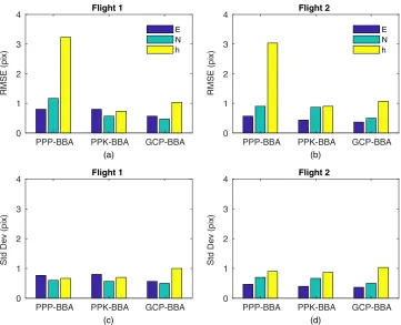
Fig. 3 displays the RMSE and standard deviation of the errors at the 24 independent check points for the PPK-BBA and PPP-BBA solutions. These are given in pixels to standardise results in terms of the expected error incurred from the GSD. Firstly, regarding the PPK-BBA solutions, check point RMSEs are better than 1 pixel in all coordinates for Flights 1 and 2 (equivalent to less than 3 cm on the ground). These results reflect the high accuracy and precision of the GPS PPK camera positions, and are similar to the check point errors obtained in comparable studies (Rehak and Skaloud, 2015; Gerke and Przybilla, 2016; Benassi et al., 2017; St€ocker et al., 2017). In addition, they also suggest that the principal distance (focal length) has been estimated with pixel-level (equivalent) accuracy for bothflights.
Considering the PPP-BBA solutions, check point RMSEs are better than 1 pixel for the northing coordinate of Flight 1 and for both the easting and northing coordinates of Flight 2, which are commensurate with the PPK-BBA results. However, a slightly larger RMSE (about 12 pixels) is observed in the northing coordinate of Flight 1. Table III shows that a 3 cm northing coordinate bias is also present in the GPS PPP camera positions of Flight 1, therefore suggesting this larger check point RMSE is likely to be caused by GPS PPP error. Both missions also exhibit large PPP-BBA height RMSEs of about 30 to 32 pixels, equivalent to 9 to 10 cm on the ground. These values are very close to the GPS PPP biases in Table III.
For the GCP-BBAs, the final RMSE values of the image residuals were 077 and 075 pixels for Flights 1 and 2, respectively, and mean 3D residuals at the GCPs were 08 and 13 cm, respectively. The GCP-BBA check point RMSEs for both Flights 1 and 2 are 1 pixel or better in all coordinate components, and thus an improvement on those of the PPP-BBA solutions, which show larger errors in northing and height for Flight 1 and height for Flight 2. This illustrates the high accuracy of the surveyed GCP coordinates.
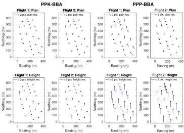
Further to the check point RMSE and standard deviation statistics, Fig. 4 shows the spatial distribution of check point errors for the PPK-BBA and PPP-BBA solutions in both planimetric and height coordinates. Planimetric check point errors in the PPK-BBA solutions generally show a random orientation, although a slight increase in magnitude towards the south of the Flight 1 image block is observed. Height check point errors are also randomly orientated, with the majority (85%for Flight 1; 77%for Flight 2) at less than 1 pixel. In comparison, planimetric check point errors in the Flight 1 PPP-BBA solution show a predominantly southerly orientation, which matches the direction of the GPS PPP camera position biases reported in Table III. For Flight 2, however, planimetric residuals are randomly orientated, as with the corresponding PPK-BBA solution. This is consistent with the centimetre-level planimetric agreement of GPS PPP and PPK camera positions in
Flight 1
(a)
PPP-BBA PPK-BBA GCP-BBA 0
1 2 3 4
RMSE (pix)
E N h
Flight 1
(c)
PPP-BBA PPK-BBA GCP-BBA 0
1 2 3 4
Std Dev (pix)
Flight 2
(b)
PPP-BBA PPK-BBA GCP-BBA 0
1 2 3 4
RMSE (pix)
E N h
Flight 2
(d)
PPP-BBA PPK-BBA GCP-BBA 0
1 2 3 4
[image:13.485.61.422.71.364.2]Std Dev (pix)
Fig. 3. Error statistics for the GPS precise point positioning (PPP), GPS post-processed kinematic (PPK) and
Table III. For both missions, the negative height-residual errors are consistent with the negative GPS PPP camera position height biases shown in Table III.
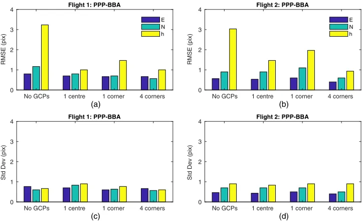
Further to the above PPP-BBA results, the effects of including one and four GCPs were investigated to see if the 3-pixel-level height RMSEs could be reduced. The four-GCP configuration comprised a GCP in each corner of the image block. For the one-GCP configuration, two runs were performed: first with a GCP in the centre of the field and second with a GCP in the far south-easterly corner of the field. These are hereafter termed one-centre-GCP and one-corner-GCP configurations, respectively. Each bundle block adjustment was parameterised as before, regarding image measurement, camera position and GCP weightings. Fig. 5 displays the RMSE and standard deviation of the errors at the (same) 24 independent check points for the PPP-BBA solutions with additional GCP configurations. The original PPP-BBA result (with no GCPs) is also shown for comparison. With the inclusion of any GCP configuration, it is seen that the check point RMSEs reduce in height, but they stay constant in the easting and northing coordinates for bothflights. The four-GCP configuration is the most effective, reducing the height error to about 1 pixel for bothflights. The one-centre-GCP configuration is shown to reduce the height error to about 10 and 15 pixels for Flights 1 and 2, respectively, whilst these values are slightly worse for the one-corner-GCP configuration at about 15 and 20 pixels. Although the one-corner-GCP configuration does not perform as well as the one-centre-GCP configuration, it still results in a 33%to 50%improvement in height RMSE. In addition to the RMSE improvements, little or negligible change is seen in the standard deviation of all three coordinate components for
0 200 400
Easting (m) 0 100 200 300 400 500 600 Northing (m)
Flight 1: Plan = 2 pix. plan res.
PPK-BBA
0 200 400
Easting (m) 0 100 200 300 400 500 600 Northing (m)
Flight 1: Height = 2 pix. height res.
0 200 400
Easting (m) 0 100 200 300 400 500 600 Northing (m)
Flight 2: Plan = 2 pix. plan res.
0 200 400
Easting (m) 0 100 200 300 400 500 600 Northing (m)
Flight 2: Height = 2 pix. height res.
0 200 400
Easting (m) 0 100 200 300 400 500 600 Northing (m)
Flight 1: Plan = 2 pix. plan res.
PPP-BBA
0 200 400
Easting (m) 0 100 200 300 400 500 600 Northing (m)
Flight 1: Height = 2 pix. height res.
0 200 400
Easting (m) 0 100 200 300 400 500 600 Northing (m)
Flight 2: Plan = 2 pix. plan res.
0 200 400
Easting (m) 0 100 200 300 400 500 600 Northing (m)
[image:14.485.63.427.70.333.2]Flight 2: Height = 2 pix. height res.
Fig. 4. Residual errors at 24 check points (denoted in each pane by the black dots) in plan (top) and height
both missions, which remain below 1 pixel. This indicates the GCPs have the effect of a datum shift on the mapping coordinates. Without the estimation of systematic error parameters at the camera positions and with little change in the camera position residuals, the GPS PPP error is expected to be absorbed by the estimated camera parameters collectively (for example, principal distance and lens distortion) and image residuals.
In summary, GPS PPP is found to have enabled high-precision (sub-pixel) photogrammetric mapping when used for direct georeferencing because of constraints placed on image orientation. Consequently, the inclusion of GPS PPP (or PPK) camera position observations in the bundle block adjustment is seen to contribute to minimising systematic errors (relating to photogrammetric aspects) at check points, with a good contribution to the block scale. Thereafter, without GCPs, remaining GPS PPP biases are shown to propagate into mapping coordinates as errors of around 10 to 12 pixels (3 to 4 cm) in plan and 3 pixels (9 cm) in height, commensurate with the magnitude of the GPS PPP camera position errors. However, with the inclusion of one or four GCPs, mapping height errors can be reduced to around 10 and 15 pixels, respectively, which is similar to thefindings of Benassi et al. (2017) and Gerke and Przybilla (2016) using relative GPS with a local reference station. As the one-GCP configurations show variable improvements, for optimal reliability it is suggested that four GCPs be used if possible, as with traditional GPS-supported aerial triangulation (for instance, Ackermann and Schade, 1993; Yuan, 2009).
Applications and Discussion
These are the first reported trials of GPS PPP for direct georeferencing on afixed-wing UAV. Without GCPs, plan-component precision and accuracy at the centimetre level has
Flight 1: PPP-BBA
(a)
No GCPs 1 centre 1 corner 4 corners 0
1 2 3 4
RMSE (pix)
E N h
Flight 1: PPP-BBA
(c)
No GCPs 1 centre 1 corner 4 corners 0
1 2 3 4
Std Dev (pix)
Flight 2: PPP-BBA
(b)
No GCPs 1 centre 1 corner 4 corners 0
1 2 3 4
RMSE (pix)
E N h
Flight 2: PPP-BBA
(d)
No GCPs 1 centre 1 corner 4 corners 0
1 2 3 4
[image:15.485.60.422.73.293.2]Std Dev (pix)
Fig. 5. Error statistics for the GPS precise point positioning (PPP) bundle block adjustment (BBA) solutions of
been obtained, commensurate with using GPS PPK, although height biases of about 10 cm were found for GPS PPP compared with centimetre-level accuracy with GPS PPK. However, the GPS PPP direct georeferencing (no GCPs) mapping accuracy and precision is still promising for a number of applications. For example, assuming similar-scale imagery, the planimetric accuracy would support the production of centimetre-level accuracy and resolution orthomosaics, as produced by Turner et al. (2014). This has utility in environmental applications such as mapping Antarctic moss beds (Lucieer et al., 2012) or in precision agriculture for locating diseased crops. The planimetric and height accuracies presented here are also commensurate with the accuracy of digital elevation models obtained in remote glacier studies (Immerzeel et al., 2014; Kraaijenbrink et al., 2016), where GCPs can generally only be located at the glacier periphery. Such a GCP distribution is unfavourable and such an application therefore favours the use of direct georeferencing. In addition, at a 120 mflying height, these check point errors are representative of an RMSE: range ratio of around 1:1200. This is better than the median value of 1:639 determined by Smith and Vericat (2015) from the analysis of 50 RMSE statistics reported in the SfM literature. Based on 2014 Royal Institution of Chartered Surveyors guidance notes (RICS, 2014), the GPS PPP-based direct georeferencing results are promising for low-accuracy topographic surveys, national urban-area mapping and geotechnical mapping (survey detail accuracy band H) although this could be extended to low-accuracy measured building surveys, boundary mapping and utility tracing with only a 5 cm height improvement (band G).
While the GPS PPP errors are substantially smaller than those found from the UAV experiments of Gross et al. (2016), further work is needed to reduce the outstanding bias of about 10 cm in height if GCPs are to be completely eliminated. Apart from having a sufficiently long flight duration to accurately estimate the ambiguity parameters, other factors affecting the height component, in particular, include antenna phase centre variation modelling, the optimum mitigation of the tropospheric delay, time-of-day geometry effects (plus the impact of observations from other GNSS constellations such as GLONASS) and resolving the ambiguities to integers. The reliablefixing of cycle slips is also a challenge in PPP positioning and an inherent limitation of GPS positioning on dynamic UAV platforms (Rehak and Skaloud, 2017a).
Conclusions and Outlook
An assessment of GPS PPP-based direct georeferencing on a fixed-wing UAV for large-scale photogrammetric mapping has been presented. Such a workflow alleviates all spatial operating constraints associated with the installation and the use of a local GPS reference station, GCPs or the need to operate within the bounds of a permanent GPS reference station network. Results are based on the analysis of two missions of 25 and 29 minutes in duration, at a flying height of 120 m, using a lightweight (~5 kg) fixed-wing UAV equipped with a digital compact camera.
variations that could not be modelled (although these also applied to the relative PPK solutions), as well as residual tropospheric delay effects.
GPS PPP camera positions were then determined by interpolating trajectories to image exposure events and applying lever-arm corrections to be used as highly weighted observations in an SfM-based bundle block adjustment using APERO image orientation software. Without GCPs, mapping errors assessed at 24 check points were revealed at the 10 to 12 pixel level in planimetric coordinates and about 3 pixels in height, but all with a precision at the 1 pixel level. Such check point residuals directly reflected the GPS PPP error magnitude and orientation, whilst the high precision indicates constraints on relative image orientation estimates, incurred from the relatively high precision of the GPS PPP camera position. Although check point height errors could potentially be improved (for example, through the use of an antenna phase centre model for the UAV antenna and further investigation of the optimum mitigation of the tropospheric delay), planimetric coordinate errors were commensurate with those obtained with a GCP-based bundle block adjustment. Applying the same workflow to a PPK-based trajectory, with integer fixed ambiguities, was shown to give check point errors at the 1 pixel level in both planimetry and height. Alternatively, with the addition of one to four GCPs, height errors resulting from the GPS PPP processing can be reduced to the centimetre level. Despite current heighting limitations, the determined precision and accuracy renders GPS PPP direct georeferencing suitable for applications such as precision agriculture and glaciology, particularly for remote operations such as alpine areas (Micheletti et al., 2015) or glacial environments (Immerzeel et al., 2014), where GCP surveys and GPS reference station installations are particularly difficult, or even dangerous, to carry out.
Acknowledgements
The authors would like to thank: QuestUAV for assistance with data collection; Martin Robertson for fieldwork support; CODE and IGS for satellite orbits and clocks; Wuhan University for the PANDA software; IGN for the APERO software; and Jing Guo and Majid Abbaszadeh for helpful discussions. Ben Grayson was supported by a UK Engineering and Physical Sciences Research Council (EPSRC) Doctoral Training Award (reference NH/110088211).
references
Ackermann, F., 1994. Practical experience with GPS supported aerial triangulation. The Photogrammetric
Record, 14(84): 861–874.
Ackermann, F. and Schade, H., 1993. Application of GPS for aerial triangulation. Photogrammetric
Engineering & Remote Sensing, 59(11): 1625–1632.
B€aumker, M.,Przybilla, H.-J.and Zurhorst, A., 2013. Enhancements in UAVflight control and sensor
orientation.International Archives of Photogrammetry, Remote Sensing and Spatial Information Sciences, 40(1/W2): 33–38.
Benassi, F.,Dall’Asta, E.,Diotri, F.,Forlani, G.,di Cella, U. M.,Roncella, R.andSantise, M.,
2017. Testing accuracy and repeatability of UAV blocks oriented with GNSS-supported aerial triangulation. Remote Sensing, 9(2): article 172. 23 pages.
Bertiger, W.,Desai, S. D.,Haines, B.,Harvey, N.,Moore, A. W.,Owen, S.and Weiss, J. P., 2010.
Single receiver phase ambiguity resolution with GPS data.Journal of Geodesy, 84(5): 327–337.
Blewitt, G., 1990. An automatic editing algorithm for GPS data.Geophysical Research Letters, 17(3): 199–
202.
Bock, H., Dach, R., J€aggi, A. and Beutler, G., 2009. High-rate GPS clock corrections from CODE:
Brown, D. C., 1971. Close-range camera calibration.Photogrammetric Engineering, 37(8): 855–866.
Cai, C. S. and Gao, Y., 2013. Modeling and assessment of combined GPS/GLONASS precise point positioning.GPS Solutions, 17(2): 223–236.
Chen, H.,Moan, T.andVerhoeven, H., 2009. Effect of DGPS failures on dynamic positioning of mobile
drilling units in the North Sea.Accident Analysis & Prevention, 41(6): 1164–1171.
Colomina, I.and Molina, P., 2014. Unmanned aerial systems for photogrammetry and remote sensing: a
review.ISPRS Journal of Photogrammetry and Remote Sensing, 92: 79–97.
Cramer, M., Stallmann, D. and Haala, N., 2000. Direct georeferencing using GPS/inertial exterior
orientations for photogrammetric applications.International Archives of Photogrammetry, Remote Sensing and Spatial Information Sciences, 33(B3): 198–205.
Deseilligny, M. P.andClery, I., 2011. APERO, an open source bundle adjustment software for automated
calibration and orientation of set of images. International Archives of Photogrammetry, Remote Sensing and Spatial Information Sciences, 38(5/W16): 269–276.
Fischler, M. A.and Bolles, R. C., 1981. Random sample consensus: a paradigm for model fitting with
applications to image analysis and automated cartography.Communications of the ACM, 24(6): 381–395.
Fraser, C. S., 1997. Digital camera self-calibration.ISPRS Journal of Photogrammetry and Remote Sensing,
52(4): 149–159.
Gerke, M.andPrzybilla, H.-J., 2016. Accuracy analysis of photogrammetric UAV image blocks: influence
of onboard RTK-GNSS and cross flight patterns. Photogrammetrie, Fernerkundung, Geoinformation, 2016(1): 17–30.
Gross, J. N., Watson, R. M.,D’Urso, S. and Gu, Y., 2016. Flight-test evaluation of kinematic precise
point positioning of small UAVs. International Journal of Aerospace Engineering, 2016: article no. 1259893. 11 pages.
Han, S., 1997. Quality-control issues relating to instantaneous ambiguity resolution for real-time GPS kinematic
positioning.Journal of Geodesy, 71(6): 351–361.
Hartley, R. and Zisserman, A., 2003. N-view computational methods. Chapter 18 in Multiple View
Geometry in Computer Vision. Second edition. Cambridge University Press, Cambridge, UK. 655 pages: 434–457.
Harwin, S.andLucieer, A., 2012. Assessing the accuracy of georeferenced point clouds produced via
multi-view stereopsis from unmanned aerial vehicle (UAV) imagery.Remote Sensing, 4(6): 1573–1599.
Heipke, C.,Jacobsen, K.and Wegmann, H.(Eds.), 2002.Integrated Sensor Orientation. Test Report and
Workshop Proceedings. OEEPE Official Publication No. 43. Bundesamt f€ur Kartographie und Geod€asie, Frankfurt am Main, Germany. 297 pages.
Heroux, P. and Kouba, J., 2001. GPS precise point positioning using IGS orbit products. Physics and
Chemistry of the Earth Part A: Solid Earth and Geodesy, 26(6–8): 573–578.
Hu, G. R.,Khoo, H. S.,Goh, P. C.andLaw, C. L., 2003. Development and assessment of GPS virtual
reference stations for RTK positioning.Journal of Geodesy, 77(5–6): 292–302.
Immerzeel, W. W.,Kraaijenbrink, P. D. A.,Shea, J. M.,Shrestha, A. B.,Pellicciotti, F.,Bierkens,
M. F. P.and de Jong, S. M., 2014. High-resolution monitoring of Himalayan glacier dynamics using
unmanned aerial vehicles.Remote Sensing of Environment, 150: 93–103.
Ip, A., El-Sheimy, N. and Mostafa, M., 2007. Performance analysis of integrated sensor orientation.
Photogrammetric Engineering & Remote Sensing, 73(1): 89–97.
James, M. R.and Robson, S., 2012. Straightforward reconstruction of 3D surfaces and topography with a
camera: accuracy and geoscience application.Journal of Geophysical Research: Earth Surface, 117(F3). 17 pages.
James, M. R.and Robson, S., 2014. Mitigating systematic error in topographic models derived from UAV
and ground-based image networks.Earth Surface Processes and Landforms, 39(10): 1413–1420.
James, M. R., Robson, S., d’Oleire-Oltmanns, S. and Niethammer, U., 2017a. Optimising UAV
topographic surveys processed with structure-from-motion: ground control quality, quantity and bundle adjustment.Geomorphology, 280: 51–66.
James, M. R., Robson, S.and Smith, M. W., 2017b. 3-D uncertainty-based topographic change detection
with structure-from-motion photogrammetry: precision maps for ground control and directly georeferenced surveys.Earth Surface Processes and Landforms, 42(12): 1769–1788.
Jozkow, G. and Toth, C., 2014. Georeferencing experiments with UAS imagery. ISPRS Annals of
Photogrammetry, Remote Sensing and Spatial Information Sciences, 2(1): 25–29.
Kouba, J.andHeroux, P., 2001. Precise point positioning using IGS orbit and clock products.GPS Solutions,
Kraaijenbrink, P. D. A.,Shea, J. M.,Pellicciotti, F.,de Jong, S. M.and Immerzeel, W. W., 2016. Object-based analysis of unmanned aerial vehicle imagery to map and characterise surface features on a debris-covered glacier.Remote Sensing of Environment, 186: 581–595.
Lagler, K., Schindelegger, M., B€ohm, J., Krasn a, H. and Nilsson, T., 2013. GPT2: empirical slant
delay model for radio space geodetic techniques.Geophysical Research Letters, 40(6): 1069–1073.
Lichti, D. D., 2002. The interpolation problem in GPS-supported aerial triangulation. The Photogrammetric
Record, 17(99): 481–492.
Liu, J.-N. and Ge, M.-R., 2003. PANDA software and its preliminary result of positioning and orbit
determination.Wuhan University Journal of Natural Sciences, 8(2B): 603–609.
Lowe, D. G., 2004. Distinctive image features from scale-invariant keypoints. International Journal of
Computer Vision, 60(2): 91–110.
Lucieer, A.,Robinson, S.,Turner, D.,Harwin, S.andKelcey, J., 2012. Using a micro-UAV for
ultra-high resolution multi-sensor observations of Antarctic moss beds. International Archives of Photo-grammetry, Remote Sensing and Spatial Information Sciences, 39(B1): 429–433.
Lucieer, A.,de Jong, S. M.andTurner, D., 2014. Mapping landslide displacements using structure from
motion (SfM) and image correlation of multi-temporal UAV photography. Progress in Physical Geography: Earth and Environment, 38(1): 97–116.
Mader, G. L., 1999. GPS antenna calibration at the National Geodetic Survey.GPS Solutions, 3(1): 50–58.
Marques, H. A.,Marques, H. A. S.,Aquino, M.,Veettil, S. V.andMonico, J. F. G., 2018. Accuracy
assessment of precise point positioning with multi-constellation GNSS data under ionospheric scintillation effects.Journal of Space Weather and Space Climate, 8: article A15. 14 pages.
Micheletti, N.,Lane, S. N.andChandler, J. H., 2015. Application of archival aerial photogrammetry to
quantify climate forcing of Alpine landscapes.The Photogrammetric Record, 30(150): 143–165.
Murtiyoso, A. andGrussenmeyer, P., 2017. Documentation of heritage buildings using close-range UAV
images: dense matching issues, comparison and case studies.The Photogrammetric Record, 32(159): 206– 229.
Nex, F.and Remondino, F., 2014. UAV for 3D mapping applications: a review. Applied Geomatics, 6(1):
1–15.
Peppa, M. V.,Mills, J. P.,Moore, P.,Miller, P. E.andChambers, J. E., 2016. Accuracy assessment of
a UAV-based landslide monitoring system.International Archives of Photogrammetry, Remote Sensing and Spatial Information Sciences, 41(B5): 895–902.
Rehak, M. and Skaloud, J., 2015. Fixed-wing micro aerial vehicle for accurate corridor mapping.
International Annals of Photogrammetry, Remote Sensing and Spatial Information Sciences, 2(1/W1): 23–31.
Rehak, M.andSkaloud, J., 2017a. Performance assessment of integrated sensor orientation with a low-cost
GNSS receiver. ISPRS Annals of Photogrammetry, Remote Sensing and Spatial Information Sciences, 4(2/W3): 75–80.
Rehak, M. and Skaloud, J., 2017b. Time synchronization of consumer cameras on micro aerial vehicles.
ISPRS Journal of Photogrammetry and Remote Sensing, 123: 114–123.
Reshetyuk, Y.and Martensson, S.-G., 2016. Generation of highly accurate digital elevation models with
unmanned aerial vehicles.The Photogrammetric Record, 31(154): 143–165.
RICS, 2014.Measured Surveys of Land, Buildings and Utilities. Third edition. Royal Institution of Chartered Surveyors, London, UK. 51 pages. http://www.rics.org/uk/knowledge/professional-guidance/guidance-notes/ measured-surveys-of-land-buildings-and-utilities-3rd-edition/ [Accessed: 25th February 2018].
Shi, J. B.,Yuan, X. X.,Cai, Y.andWang, G. J., 2017. GPS real-time precise point positioning for aerial
triangulation.GPS Solutions, 21(2): 405–414.
Smith, M. W. and Vericat, D., 2015. From experimental plots to experimental landscapes: topography,
erosion and deposition in sub-humid badlands from structure-from-motion photogrammetry.Earth Surface Processes and Landforms, 40(12): 1656–1671.
Stocker, C.€ ,Nex, F.,Koeva, M.andGerke, M., 2017. Quality assessment of combined IMU/GNSS data
for direct georeferencing in the context of UAV-based mapping.International Archives of Photogrammetry, Remote Sensing and Spatial Information Sciences, 42(2/W6): 355–361.
Turner, D.,Lucieer, A.andWatson, C., 2012. An automated technique for generating georectified mosaics
from ultra-high resolution unmanned aerial vehicle (UAV) imagery, based on structure from motion (SfM) point clouds.Remote Sensing, 4(5): 1392–1410.
Turner, D., Lucieer, A. and Wallace, L., 2014. Direct georeferencing of ultrahigh-resolution UAV
Wackrow, R. and Chandler, J. H., 2008. A convergent image configuration for DEM extraction that minimises the systematic effects caused by an inaccurate lens model. The Photogrammetric Record, 23(121): 6–18.
Yastikli, N.andJacobsen, K., 2005. Direct sensor orientation for large scale mapping–potential, problems,
solutions.The Photogrammetric Record, 20(111): 274–284.
Yu,X. and Gao, J., 2017. Kinematic precise point positioning using multi-constellation global navigation satellite system (GNSS) observations.ISPRS International Journal of Geo-Information, 6(1). 15 pages.
Yuan, X. X., 2009. Quality assessment for GPS-supported bundle block adjustment based on aerial digital
frame imagery.The Photogrammetric Record, 24(126): 139–156.
Yuan, X., Fu, J. H., Sun, H. X. and Toth, C., 2009. The application of GPS precise point positioning
technology in aerial triangulation.ISPRS Journal of Photogrammetry and Remote Sensing, 64(6): 541–550.
Zumberge, J. F.,Heflin, M. B.,Jefferson, D. C.,Watkins, M. M.andWebb, F. H., 1997. Precise point
positioning for the efficient and robust analysis of GPS data from large networks.Journal of Geophysical Research–Solid Earth, 102(B3): 5005–5017.
Resume
L’implementation du positionnement ponctuel precis (PPP) par systeme de positionnement global (GPS) sur un dronea voilurefixe est appliqueea la cartographie photogrammetrique avec des precisions de l’ordre du centimetre en planimetrie et 1 decimetre en altimetrie,a partir de vols d’une duree de 25a 30 minutes. Les positions de l’instrument de prise de vue estimees par PPP GPS sont utilisees pour contraindre l’estimation des positions des images lors de l’ajustement des faisceaux photogrammetriques, comme avec un position GPS relatif. Le PPP GPS permet de rel^acher toutes les contraintes operationnelles de nature spatiale liees a l’installation eta l’utilisation de points d’appui au sol ou d’une station GPS locale de reference, ou encorea la necessite d’operer dans les limites d’un reseau de stations GPS permanentes. Cela simplifie la logistique operationnelle et permet une cartographie photogrammetrique a large echelle m^eme dans les situations geographiques les pluseloignees et les plus difficiles.
Zusammenfassung
Die Anwendung von Precise Point Positioning (PPP) des Global Positioning Systems (GPS) wird am Beispiel einer photogrammetrischen Kartierung mit Fl€ugen von 25–30 Minuten Dauer mit einem Starrfl€ ugel-UAV (unmanned aerial vehicle) demonstriert. Es werden cm-Genauigkeiten in der Lage und 1 dm-Genauigkeiten in der H€ohe erzielt. Die durch GPS PPP gesch€atzten Projektionszentren der Kamera werden als Zwangsbedingungen f€ur die Sch€atzung der Bildpositionen in der photogrammetrischen B€undelausgleichung aus relativen GPS Positionierungen eingef€uhrt. Mit GPS PPP werden alle operationellen Einschr€ankungen verringert, die mit der Erstellung und Nutzung von Passpunkten, einer lokalen GPS Referenzstation oder der Notwendigkeit innerhalb der Grenzen eines permanenten, regionalen GPS Referenzstationsnetzes zu operieren verbunden sind. Damit wird die Betriebslogistik vereinfacht und eine großmaßst€abige photogrammetrische UAV Kartierung wird sogar in den entlegensten und anspruchvollsten geographischen Orten durchf€uhrbar.
Resumen
de operar dentro de los lımites de una red permanente de estaciones de referencia GPS. Esto simplifica la logıstica operativa y permite aplicaciones fotogrametricas a gran escala con vehıculos aereos no tripulados incluso en condiciones desafiantes como ubicaciones geograficas remotas.
摘要
本文以案例展示应用全球定位系统(GPS)精密单点定位(PPP)用于固定翼无人机(UAV)的摄影测量,其
精度在水平方向可达厘米级,高程方向达分米级,飞行时间为25至30分钟。由GPS PPP所获得之摄影站坐标, 如同使用GPS相对定位得到的一样,在摄影测量光束法平差中用以约束投影中心位置。GPS PPP减轻了限制