Distribution of Control Resources in the Metasystem of Stochastic Regulators

(1)

Distribution of Control Resources in the Metasystem of

Stochastic Regulators

A.M. Pishchukhin

*

_{, T.A. Pishchukhina}

Department of Control and Informatics in Technical Systems, Aerospace Institute of Orenburg State University, Russian Federation

Abstract

The paper deals with the solution of the optimal reallocation of control resources in the metasystem of stochastic controllers, as that can be read in conjunction functioning technology of manufacturing products within the range of the enterprise. In this theoretical solution to this problem is possible only for Markov processes with a normal distribution of output indices regulators values (for example, the volume of production, the quality of manufactured products). It is proved that the variances between the controlled variables in the metasystem, and virtual work needed to support them, there is a hyperbolic dependence. Connecting a finite state machine that distributes control resources proposed in the algorithm removes the restriction of Markov processes. Perhaps finding the minimum total variance even multiplies regulators.

Keywords

Markov Processes, the Allocation of Control Resources in the Metasystem, the Total Variance of Variables Controlled, the State Machine, Resource Allocation Algorithm

1. Introduction

Managing a modern enterprise is impossible without objective timely information and optimization of

management decisions based on it. Such tasks are entrusted to the MES system / 1-10 /. Planning in such systems is usually carried out by combining the optimization heuristic with the simulation model based on information processing in stochastic production conditions / 11 /.

As shown in [12], the metasystem approach to enterprise management can be quite constructive. Considering the enterprise as a metasystem of jointly functioning technologies, let us turn to the solution of the problem of optimal allocation of control resources between them. In the MES system, this function is performed by the RAS (English Resource Allocation and Status) subsystem. Metasystem (the enterprise) is conveniently represented as a set of stochastic regulators. Accuracy of indicators produced volume and quality values for each product and each respectively technology, as well as the overhead of its achievement - specific. Since resources are always limited by their need to invest cumulatively, and not "spread" evenly across all technologies. The criterion in this case can serve as the total variance of the main indicators.

2. Theory

(2)

∑

∑∑

= = =

=

∂

⋅

+

∂

⋅

+

∂

n k n k n

m km k m k

k

Y

t

_y

f

b

Y

t

_y

f

_y

a

t

f

1 1 1

2

0 )

,

(

2

1 )

,

(

. (1)

where

f

- density of the random variable - output parameter control,

a

_k

(

Y

,

t

)

- the drift coefficient,

b

_km

(

Y

,

t

)

- diffusion coefficient, depending on the vector of phase coordinates

Y

of control and time

t

.

Control action falls into the right side of the equation and makes it inhomogeneous. It is necessary to determine the optimal control actions for normal probability distribution.

The decision transformed the inhomogeneous equation (1) can be expressed in terms of the Green's function

( )

(

) ( )

,

4 exp

2

1 )

exp(

,

0 2 2

x

p

bt

u

t

dtd

y

bt

y

b

a

t

b

a

t

Y

f

_∫∫

∞

∞ − ∞













₋

−

=

(2)

where

u

( )

x

,

t

- the control action.

Considering the probability density obeys the normal distribution, and substituting into the left side of the control solution desired result (in the form of the probability density of the Gaussian), we obtain Fredholm equation of the 1st kind

(

)

(

x

_{) ( )}

_x

p

σ

p

σ

bt

u

t

dtd

y

bt

y

b

a

t

b

a

y

уст

_,

4 exp

2

1 )

exp(

2 exp

2

1

0 2 2 2 2

∫∫

∞ ∞ − ∞













₋

−

=













−

. (3)

With the help of this equation we can study the dynamics of the control system. We restrict ourselves to the study of steady motion. To do this, return to the equation (1) for the one-dimensional case with constant coefficients, a and b, remove the derivative with respect to time and substitute instead of the probability density of normal distribution:

)

(

)

(

2 )

(

2

1

₂ 2

) ( 3

3 2

5

y

e

u

y

a

b

y

b

y yуст

уст





⋅

=





₋

− − σ

σ

p

, (4)

where yуст - regulator setting, u (y) - control action.

We introduce the concept of virtual work as the work required to make the control system to maintain the dispersion of the output value at a given level

( )

u

( )

y

e

dy

A

ус y y 2 2 σ 2 ) (

π

2 σ

1 σ

− − ∞ ∞ −

∫

=

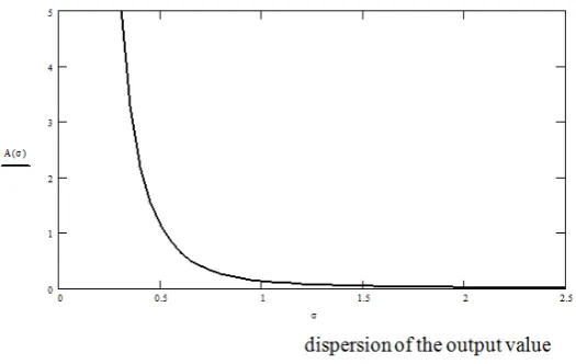
. (5)

[image:2.595.179.442.558.724.2]

Using the formula (4), you can plot the dispersion of the output value of the virtual work, having hyperbolic, inexplicable nature of the process (see. Figure 1).

Figure 1. The dependence of the dispersion from virtual work

(3)

the controlled quantity to an arbitrarily small value (But not to zero). Conversely, reducing the resources allocated to the control, we arrive at the dispersion increase up to infinity.

Having controlled depending on the magnitude of the dispersion from the virtual work can be optimally allocate resources. Classic optimization criterion is usually taken in the following form [14]

( )

(

,

)

(

)

]

[

)]

,

(

[

1 1

0

M

l

Y

t

M

L

Y

τ

u

τ

K

u

τ

d

τ

I

k

o

t

T

k

+

∫

+

−

=

, (6)

where L (Y, t), l1 (Y, tk) - given positive definite functions, K - symmetric positive definite or diagonal matrix of positive

factors.

Considering the functional reflecting losses in the metasystem, we assume that

l

₁

(

Y

,

t

_k

)

= 0, the function

L

does not depend on controllable variables, but on their variances, and instead of the normal operation control actions used virtual work:

∑ ∫

= ∞













+

=

n i t i i

i

t

A

t

dt

M

I

1 ₀

))

),

(

)

(

α

σ

. (7)

Solving the problem of optimal control of a metasystem with this functionality, it is possible to determine the optimum meaning of dispersion of the output values. To solve this, in conjunction system including equation (4), determining (5) and the criterion (7)

(

)

(

)

(

)

(

)

[

]











→

+

=













−

∑

∫

= ∞ ∞ − − − − −

.

min

)

(

,

1 ,

2 )

(

)

(

),

(

2

1

1 2 2 3 3 2 \ 5 2 2 2 2 n

i i i i i

y y i i i i i i y y уст i i i i уст i i

A

n

i

dy

e

y

u

A

y

u

e

y

a

b

y

b

уст уст

σ

α

p

σ

p

σ σ



(8)

Differentiating the last equation at all

σ

i, and equating the derivative to zero, we obtain a new system of n equations. In it

we substitute the expression of virtual work of the second equation (8), which, in turn, substituted control action from the first equation (8). Finally we get n equations to find the optimal parameters of stochastic variance output regulators

n

i

dy

e

y

a

b

y

b

i y y уст i i i i уст i i i i уст

,

,1

2 )

(

2 )

(

2

1

2 2 ) ( 3 3 2 5



=

−

=





























−

∂

∫

∞ ∞ − − −

pα

σ

σ . (9)

3. Method

Solving systems of obtained equations determines the optimal values for the variances of each regulator. However, not always sufficient information for solving the system of equations obtained. Further control can be reduced to the finite state machine, which will reallocate resources to control "wealthy" systems in the metasystem to "dysfunctional" (i.e., those dispersion of output values for which has increased the most). All versions of the distribution of control (finite state machine) can be described by the following matrix:





















−

∆

−

∆

−

=

∆

,...,

,

,...,

,

,...,

,

2 1 2 21 1 12 n n n n

u

U

(4)

Here, the column numbers correspond to the number of systems within the metasystem, with which control resources "removed", and line numbers correspond to the number of systems which control actions are directed. Dash marked unused condition.

This decision is unfair for multi system. Let us consider the redistribution of resources. As proved above hyperbolic dependence of the dispersion of virtual work (see. Figure 1), assume for simplicity of analysis, that this dependence has two controlled variables

Α

=

Α

=

α

σ

β

σ

₁

,

₂ , (11)

where

α

,

β

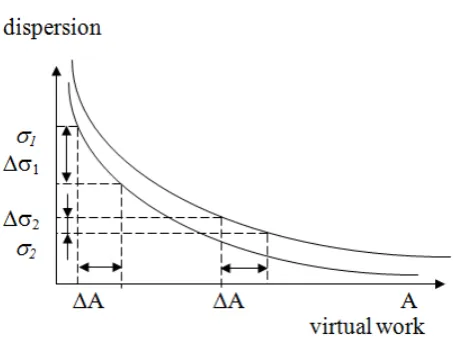
- dimensional coefficients.

[image:4.595.66.293.273.449.2]

Schedule of dependency is illustrated in Figure 2.

Figure 2. Scheme of control resource reallocation

Control is necessary to conduct such a way that the total variance was minimal

∑

=

→

=

N i i

K

1

min

σ

(12)

It is possible to carry out a two-level control with adjusting control parameters to optimal values, and then, using coordinated control actions to minimize the criterion K [15]. Taking a small fraction of the resource by the second parameter and putting it into the first improvement, we will get a deduction of two dispersions of controlled variables on the value

2

1

σ

−

∆

(13) Such a redistribution of resources rationally, yet this difference is positive. Equality weaned and added resources give an equation for finding the optimal points

σ

₁*

,

σ

₂*

2 * 2 * 1 1

σ

β

σ

β

σ

α

σ

α

₋

₌

₋

(14)

Introducing the notation for the initial sum

C

=

+

2 1

σ

β

σ

α

it can be expressed in one optimum value through other

α

σ

β

σ

−

=

_* 1 * 1 *

2

_C

(15)

The goal of optimization is now formulated as follows:

min

* 1 * 1 *

1



→











−

+

α

σ

β

σ

C

(16)

Taking the derivative of this sum with respect to σ1* and

equating it to zero, we find the optimal value

( )

(

)

(

)

.

;

0

2

* 1 2 * 1 * 1 2 * 1 2

C

αβ

α

σ

α

σ

α

β

α

ασ

σ

±

=

−

(17)

Considering the factors

α

>

1

and

β

>

1

taking into account that

σ

₁* is always positive-enforcement, we have a unique solution











+

=

+

=

.

;

* 2 * 1

C

αβ

β

σ

αβ

α

σ

(18)

The minimum sum is

(

)

C

2 * 2 * 1

β

α

σ

+

=

+

(19)

If we required optimal match points, the equation (14) would take the form:

2 * * 1

σ

β

σ

β

σ

α

σ

α

₋

₌

₋

(20) His decision

(

)

1 2 2 1 *

βσ

ασ

σ

β

α

σ

+

=

(21)

The minimum sum is 2σ*_.

Determining the difference between the two minimum sums, we see that it is positive

(

)

(

)

(

)

₀

(5)

parameters are satisfied with the system designer, it is possible to successively adding the danger of deviations following parameters define a unique value nearly optimal

σ*_{and the minimum sum}

.

* 1

*

_σ

σ

N

N i i

=

∑

=

(23)

Finding the difference between this value σ*_{with every}

danger of deviation can be achieved separately by channel control systems belonging to the metasystem.

If, however, this difference does not suit us, then spend more subtle study. Obviously, redistribution of control resources can be stopped when the difference (13) is equal to 0.

Restricting end increments

;

1 1

_∂

_Α

∆Α

∂

=

∆

σ

2

,

2

_∂

_Α

∆Α

∂

=

∆

σ

(24)

we see that the effect of the redistribution of resources is proportional to the partial derivatives. In such case the following algorithm can be arranged.

1. Calculate the partial derivatives of the variances of all control resource values for the data points (σ1, σ2…σN).

2. Sort derivatives in descending order.

3. Reallocate resources ΔA value of the parameter control with a maximum value of the derivative on the control parameters with a minimum of the derivative.

4. Calculate the derivatives that have changed as a result of step 3.

5. Determine the maximum difference of derivatives (max-min), and if it exceeds a certain value δ, go to step 2.

6. End of Work.

Value δ defined here for the minimum change in the derivative on the edge of the range for a given change in the resource ΔA. This algorithm is more accurate than ΔA smaller. However, it increases the time it works.

Thus, when carrying out such coordination, we reduce the sum dispersion controlled variables to a minimum or can save resources of control actions (depending on what is more favorable).

4. Data and Modeling Results

A meta-model consisted of three parallel operating control characterized by systematic error ai and standard spread

i

b

, where i = 1,2,3. The change in time density distribution of a controlled value obeys the Fokker-Planck-Kolmogorov

i i

i i i

i i

i

_u

y

b

y

a

t

∂

=

∂

−

∂

+

∂

2 2

2 ω

ω

, (25) where yi -control value, ui - control action, modifying the

accuracy of controls (for adjustment).

The above decision was carried out for tasks continuously controlled dispersion. However, in practice, the regulators for adjustment are carried out in a pulse mode, that is, from time to time. Substituting impulse action to the right side of the equation (25), we find its solution

(

)













₋

−

=

t

b

y

t

b

t

b

a

y

b

a

i i mo i i

i i i i i i

4 exp

2

1 )

exp(

2 2

p

ω

.

(26) As you can see, the resulting solution is a normal law with standard deviation (SD) time-varying (depending only on the parameter

b

i) and demolition at yi-axis (depending only on

i

a

).

Standard deviation averaged over a certain period of time, you can compute using the following formula:

(

)

(

T

t

)

t

b

T

b

d

b

t

T

i i

T t

i

ср

₋

−

=

−

=

_∫

3

2

1 _τ

_τ

σ

. (27)

Impulse control process is simulated on a computer with the following parameters:

a

=1,

b

=1,

y

_mo=1,

σ

_ср=1.

In the absence of control influences the measured value density distribution is subject to demolition and blur, as shown in Figure 3.

(6)

[image:6.595.108.502.124.311.2]

Figure 3. Blur controlled quantity of the probability density in the absence of the adjustment

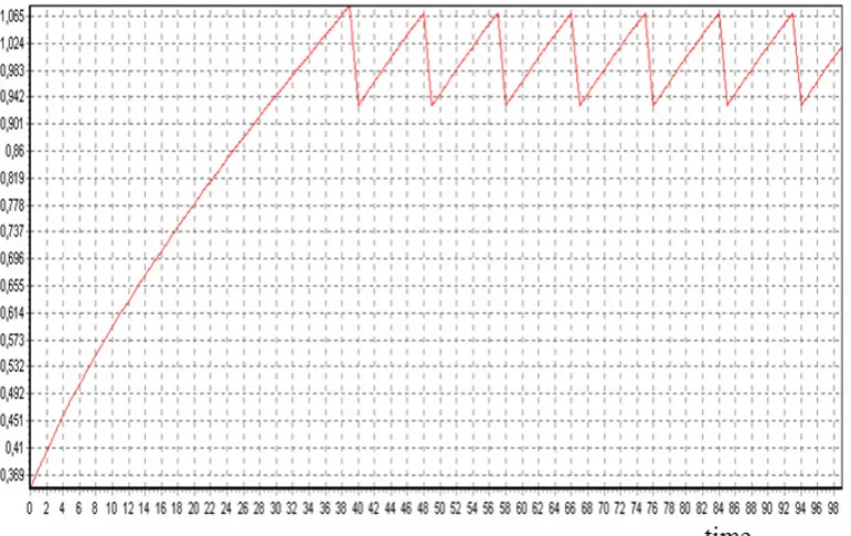
Figure 4. Changing the standard deviation over time when pulse the adjustment

[image:6.595.115.501.367.610.2]

(7)

[image:7.595.113.497.125.353.2]

Figure 5. Dependence of virtual work on the duration of the period between the adjustments

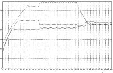
Figure 6. Changes dispersions three controllers during the experiment

Breaks in the graph are due to hit the whole number of periods in the estimated time. It follows from this dependency, a minimum total virtual work occurs with

[image:7.595.111.499.432.685.2]

(8)

dramatically.

If the metasystem is multiply rather than multidimensional as in the previous study, the problem is not amenable to analytical solution.

In this case it is necessary to synthesize the state machine, which uses the algorithm described in the previous section, and its operation will determine the optimal values of dispersions of controlled variables.

A multiply modeled here as follows. Counting-out that the second and third regulators have a positive impact on the first one (level overflow control actions everywhere assumed to be equal to 10%). The first and second controllers adversely affect a third. Finally, the first controller has a positive effect on the second and the third - negative. The results of this experiment are shown in Figure 6.

The chart is divided into three areas. The first - an area of independent work of regulators (the dispersion increases in all three channels are the same). In the second region introduced as described above controls the relationship that leads to an increase of the controlled quantity of the dispersion in the third regulator, the first reduction and almost no change in the dispersion of the second controller. The third area includes a state machine that is optimally redistributing control actions, dispersions returns almost the same of their value.

5. Discussion

From the experimental modeling of metasystem is seen that, although the behavior of its constituent systems described by the Fokker-Planck-Kolmogorov, we have different ways to control them. In the second case, you can directly increase the frequency of inclusions in cases of great uncertainty, and in the first you can only create the conditions for reducing the quantities of controlled dispersions.

6. Conclusions

Thus, the criterion as the sum of the variances of controlled variables and virtual work required to maintaining these dispersions, to optimize the control in metasystem, minimizing the virtual work and maintaining acceptable control accuracy in separate systems (controllers).

Variances between the controlled variables in the metasystem, and virtual work needed to support them, there is a hyperbolic dependence.

When pulse control metasystem with decreasing frequency pulse impact virtual work, directed at the maintaining of the specified dispersions controlled variables, increases dramatically. Minimality virtual work takes place under continuous management.

In the case of a multiply metasystem need a model of a finite automaton, operating on a special algorithm and allows

"automatically" find the optimal values of the variances of output values.

REFERENCES

[1] Jonathan Kall. Manufacturing Execution Systems: Leveraging Data for Competitive Advantage. https://www.qualitydigest.com/aug99/html/body_mes.html. [2] Joseph A. Vinhais Manufacturing Execution Systems: The

One-Stop Information Source.

https://www.qualitydigest.com/sept98/html/mes.html. [3] Xiaopan Gao, Ruisheng Zhang, Yan Zhang, Shui Jing

Research Focus on MES Oriented Communication among Enterprise Informatization System. Asia-Pacific Conference on Services Computing. 2006 IEEE (2012) pp.: 365-368 DOI Bookmark:

http://doi.ieeecomputersociety.org/10.1109/APSCC.2012.72 [4] Byeong Woo Jeon, Jumyung Um, Soo Cheol Yoon & Suh

Suk-Hwan. An architecture design for smart manufacturing execution system// Computer-Aided Design and Applications. Volume 14, 2017 - Issue 4 Pages 472-485

[5] Eric A. Marks Manufacturing Execution Systems: Enablers for Operational Excellence and the Groupware for Manufacturing // Information Strategy: The Executive's Journal Volume 13, 1997 - Issue 3 Pages 23-29

[6] Theodor Borangiu, Silviu Răileanu, Thierry Berger & Damien Trentesaux Switching mode control strategy in manufacturing execution systems //International Journal of Production Research Volume 53, 2015 - Issue 7 Pages 1950-1963

[7] B. Saenz de Ugarte, A. Artiba & R. Pellerin Manufacturing execution system – a literature review // Production Planning & Control. The Management of Operations. Volume 20, 2009 - Issue 6: Complex Systems Analysis, Modelling and Simulation. Pages 525-539

[8] Silviu Raileanu , Theodor Borangiu , Octavian Morariu, Octavian Stocklosa ILOG-based mixed planning and scheduling system for job-shop manufacturing 2014 IEEE International Conference on Automation, Quality and Testing, Robotics (AQTR) (2014) Cluj-Napoca, Romania May 22, 2014 to May 24, 2014, pp.: 1-6

[9] Yan Ping Zhou //Design of Manufacturing Execution System in Tire Enterprises// Applied Mechanics and Materials (Volumes 411-414) p.2343-2346

DOI10.4028/www.scientific.net/AMM.411-414.2343 [10]Zhi Hui Huang, Shu Lin Kan, Liang Wen Yan, Jun Li, Qi

Hong Chen Advanced Materials Research (Volumes 179-180) p.1356-1363 DOI10.4028/www.sci-entific.net/AMR.179-180 .1356

(9)

[12]Pishchukhin A.M., Pishchukhina TA The Control Simulation of the Enterprise on the Basis Metasystem Approach // Universal Journal of Control and Automation. 2013. Vol. 1 (4). P 98-102.

[13]Volkov IK Zuev SM, Tsvetkova GM Random processes.-

Moscow: Publishing House of the MSTU. Bauman, 1999.- 448 p.

[14]Manual control theory. -M.: Nauka. 1987.-712 p.