Pull in Effect for Micro Beam with Tensile Force

(1)

Pull-in Effect for Micro Beam with Tensile Force

Skubov D. Yu.1,2,*, Privalova O. V.2, Shtukin L. V.1,2

1

Institute of Problem of Mechanical Engineering RAS & Saint-Petersburg, Russia 2

Department of Mechanics and Processes of Control, Peter the Great St. Petersburg Polytechnic University, Russia

Abstract

Recent time the development and

achievement of micro- and nano-electromechanical systems (MEMS and NEMS) are appeal the great interest of physics, biologists, engineers-electricians. The designing of MEMS based on pull-in effect consists in interaction of electrostatic field with thin elastic conductive beam. This interaction leads to pull-in instability – the effect of collapse of two initially parallel conductive layers, which play the role of capacitor. The important significance of MEMS have been acquired [1, 2] such, for example, as micro-switches with forward or rotary movement. These devices may be membrane else cantilever or another type, also high speed rotational actuator – contactless micro-gyroscope.

Keywords

Pull-in Effect, Electrostatic Field, Micro-beam

1. Introduction

The «history» of pull-in effect is very long. The full description of this study we can find in work of J. Pelesko and T. Driscoll [3]. In this article the investigation of influence of the edge effect of distributed electric field on the equilibrium forms of conductive membrane – upper plate of drum-shaped electrostatically actuating MEMS device was fulfilled. Also we can mention work of Sl. Krylov et al. [4] in which the analysis of the influence of initially curved beam on the pull-in effect of micro beam loaded by distributed electro-static force is studied. It gives us the criteria to predict action of non-symmetric buckling in electrostatic field on constitution of the bistable forms of micro beam. The main purpose of our article is to give estimation of the relation between flexural stiffness arising due to tension of micro-rod and bending stiffness of this electro-elastic system.

Free Oscillation. Eigen Frequency and Modes

Here effect of «pull-in» instability is considered for beam with tensile force. «Pull-in» instability is an inherently

nonlinear effect connected with disappearance of equilibrium forms of elastic part of sensitive or actuating mechanism, which in our task is considered as a flexible double clamped microbeam. Its parameters are: length

𝑙

, bending stiffness

𝐸𝐼

,

tensile force

𝑃

,

𝜌𝐹

– the density on the unit of length. Moreover we suppose that the bending stiffness is much less than the stiffness of string. This assumption gives us the possibility to build the asymptotic approximation of pull-in branching curve and estimate the influence of stiffness relation.

[image:1.595.308.534.383.496.2]

1 – elastic element, 2 – isolate support, 3 - motionless electrode, 4 - voltage source

Figure 1. Model of investigation

In static equation of beam taking in account the tensile force 𝑃> 0 has a next form

𝐸𝐼𝑦𝐼𝑌_{− 𝑃𝑦}′′₊_{𝜌𝐹𝑦̈}_{= 0} ₍₁₎

where 𝑦 – deflection, 𝑦𝐼𝑉 =𝑦′′′′=𝜕4𝑦

𝜕𝑥4,𝑦′′=𝜕 2_𝑦 𝜕𝑥2, 𝑦̈= 𝜕2_𝑦

𝜕𝑡2, 𝑥 ∈[0,𝑙], 𝑃=𝐸𝑆 Δ𝑙

𝑙 – longitudinal tensile load with

the double-clamped boundary conditions:

𝑦(0) =𝑦(𝑙) = 0, 𝑦′_{(0) =}_𝑦′₍_𝑙_{) = 0.} ₍₂₎

The eigen frequency of the flexural oscillations has a scale factor Ω₀=1

𝑙� 𝑃

𝜌𝐹 . Let’s introduce the

dimensionless variables 𝑠=𝑥_𝑙, 𝜏=Ω₀𝑡 and non-dimensional buckling 𝑤=𝑦/ℎ (ℎ – magnitude of gap).

The equation (1) can be written in the form:

(2)

where the dimensionless parameter 𝜀𝛼= 𝐸𝐼

𝑃𝑙2 and 𝜀= ℎ 𝑙

are introduced (further believed small).

At first let’s consider free harmonic oscillation, assuming that 𝑤=𝑊(𝑠)𝑒𝑖Ωτ, here Ω −eigen frequency. We obtain the homogeneous differential equation:

𝜀𝛼𝑊𝐼𝑌_{− 𝑊}′′_{− Ω}2_𝑊_{= 0}₍₄₎

Believing that 𝑊=𝐶𝑒𝜆𝑠 we obtain the dimensionless characteristic biquadratic equation

𝜀𝛼𝜆4_{− 𝜆}2_{− Ω}2_{= 0,}₍₅₎

which has two roots: 𝜆₁2_,₂= 1

2𝜀𝛼± 1

2𝜀𝛼√1 + 4𝜀𝛼Ω2 .

These roots can be separate in two groups: positive and negative. Let’s input designations

𝜈=� 1

2𝜀𝛼 ��1 + 4𝜀𝛼Ω2−1� ,

𝜅=�_2𝜀𝛼1 (√1 + 4𝜀𝛼𝛺2_{+ 1)}_{. (6)}

The solution of equation (4) can be written in the form:

𝑊𝑖=𝐴𝑠𝑖𝑛𝜈𝑠+𝐵𝑐𝑜𝑠𝜈𝑠+𝐶𝑠ℎ𝜅𝑠+𝐷𝑐ℎ𝜅𝑠 (7)

Based on the boundary condition the eigen modes and frequency are determined from homogenous algebraic system:

𝐵+𝐷= 0, ν𝐴+𝜅𝐶= 0,

Asin𝜈+𝐵cos𝜈+𝐶𝑠ℎ𝜅+𝐷𝑐ℎ𝜅= 0, (8)

νA cos𝜈 − 𝜈𝐵sin𝜈+𝜅𝐶𝑐ℎ𝜅+𝜅𝐷𝑠ℎ𝜅= 0.

Having used system of equation (8) we obtain the characteristic equation

2𝜈𝜅(cos𝜈ch𝜅 −1) + (𝜈2_{− 𝜅}2_{) sin}_𝜈_sh_𝜅_{= 0}_{, (9)}

where 𝜈𝜅= Ω�1

𝜀𝛼 , 𝜈2− 𝜅2= − 1

𝜀𝛼 . From (9) we

find the eigen frequencies Ω_𝑖 , 𝑖= 1 , 2, . .. The modes of free oscillations 𝑊_𝑖 corresponded to 𝑖 eigen frequency has a form

𝑊𝑖(𝑠) = 𝐴𝑖(sin𝜈𝑖𝑠 − 𝐺𝑖cos𝜈𝑖𝑠 − _𝜅𝜈𝑖_𝑖 sh𝜅𝑖𝑠+𝐺𝑖ch𝜅𝑖𝑠),

(10) Here 𝐺_𝑖= sin 𝜈𝑖−

𝜈𝑖 𝜅𝑖sh 𝜅𝑖

cos 𝜈𝑖−ch 𝜅𝑖 . The coefficients 𝐴𝑖 is

determined from condition of orthonormality

∫ 𝑊₀1 𝑖 (𝑠)𝑊𝑘(𝑠)𝑑𝑠= 𝛿𝑖𝑘.

Table1. The some results of calculation are shown

𝜀𝛼 Ω1 Ω2 Ω3

0.01 4.10 9.12 15.60

0.1 7.78 20.65 39.50

0.2 10.60 28.44 54.98

Figure 2. The first two symmetric eigen-modes

2. Electrostatic Field

The electrostatic forces are obtained from the expression of electrostatic potential. The distribution of this potential between electrodesΨ(𝑥,𝑧) is determined from Laplace’s equation

∆Ψ= 0 (11) Further we consider only symmetric case of conductive layer deformation. One (upper) layer has an electric potential 𝑉 lower and other sidewalls have zero potential, believing that side walls are separated from conductive layer by thin insulating layer. The boundary conditions in this case have a form:

𝑥= 0; Ψ= 0, 𝑥=1_{2 ;}𝜕Ψ_𝜕𝑥 = 0.

𝑧=ℎ; Ψ=𝑉, 𝑧= 0; Ψ= 0 (12) Let’s introduce dimensionless coordinates 𝜉=2𝑥

𝑙 ,𝜁= 𝑧/ℎ . The non-dimensional expression for potential

𝜓=Ψ/𝑉 satisfies to the same equation (11).

The calculation of electric field is fulfilled taking in account the edge effect, assuming that the ratio of gap value ℎand length of layer 𝑙 (𝜀=ℎ

𝑙) is small. Having

(3)

boundary task relatively 𝜓�, believing that 𝜓=𝜓�+𝜁

𝜀2 𝜕2𝜓� 𝜕𝜉2 +𝜕

2_𝜓�

𝜕𝜁2 = 0 or 𝜕 2_𝜓� 𝜕𝜂2+𝜕

2_𝜓�

𝜕𝜁2 = 0 (13)

with boundary conditions:

𝜉= 0(𝜂= 0), 𝜓�=−𝜁;

𝜉= 1, 𝜕𝜓_𝜕𝜏�= 0, (14)

𝜁= 0, 𝜓�= 0; 𝜁= 1, 𝜓�= 0.

Using symmetry of electroelastic system, all subsequent relations will be written only for its left half (𝜉= 2𝑠, 0≤

𝑠 ≤0.5, 0≤ 𝜉 ≤1). The solution of boundary task (13), (14) is searched by method of boundary layer 𝜓�=

𝜓�0(𝜂,𝜉) +𝜀𝜓�1(𝜂,𝜉,𝜀) . In a case of non-deformed

plate-layer the expression of electrostatic potential has an approximated view:

𝜓=𝜁+_𝜋2∑∞ (−1_𝑛)𝑛

𝑛=1 exp�−𝜋𝑛𝜉_𝜀 �sin𝜋𝑛𝜁. (15)

Taking into account the beam deflection (upper plate of «capacitor») 𝑤(𝑠) the electric potential is determined by expression:

𝜓=_𝑢₍𝜁_𝜉_{) +}2_{𝜋 �}(−_𝑛1)𝑛

∞

𝑛=1

exp�−𝜋𝑛𝜉_{𝜀 �}sin𝜋𝑛𝜁,

𝑢(𝜉) = 1− 𝑤(𝜉) (16) The distribution of potential 𝜓 is shown in Fig.3.

Figure 3. Distribution of electrostatic potential and electric intensity (𝜀= 0.1)

The distributed force of attraction acts in a normal of upper layer (Γ) can be found by expression:

𝑓(𝑠) =�𝜀2₍𝜕𝜓 𝜕𝜉)2+ (

𝜕𝜓

𝜕𝜁)2�_Γ, 𝜁Γ= 𝑢(𝑠) = 1− 𝑤(𝑠).

(17) Differentiating electro potential on 𝜉 we obtain

𝜕𝜓 𝜕𝜉 =

𝜁𝑤′ 2(1−𝑤)2−

2

𝜀∑∞𝑛=1(−1)𝑛exp (− 2𝜋𝑛𝑠

𝜀 )sin 𝜋𝑛𝜁 . (18)

Here and future we will neglect the first item

containing 𝜀2 in expression (17). Also in future we will neglect the changing of normal of the bounding upper elastic layer that leads to 𝜁= 1.So electric force acting in a normal to elastic layer can be calculated using the expression

𝑓(𝑠) = (𝜕𝜓_𝜕𝜁)2_,𝜕𝜓 𝜕𝜁 =

1 1−𝑤+𝑆, 𝑆= 2∑∞ exp�−2𝜋𝑛𝑠_𝜀 �

𝑛=1 . (19)

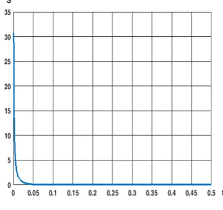
[image:3.595.311.529.225.430.2]

The dependence 𝑆(𝑠) for left half of our system is shown in Fig.4

Figure 4. Description of edge effect

So we can see very fast decay of edge effect.

3. Electro-elasticity

The task of electro-elasticity consist from static equation of beam flexure under of action the electric force has a form

𝜀𝛼𝑤𝐼𝑉_{− 𝑤}′′₌_𝛾2_𝑓₍_𝑠_,_𝑤_),₍₂₀₎

where 𝛾2=𝜖_2𝑃ℎ0𝑉2𝑙₃2 ( 𝜖₀ –dielectric permittivity) and homogeneous boundary conditions

𝑤(0) = 0,𝑤′_{(0) = 0,}_𝑤_{(1) = 0,}_𝑤′_{(1) = 0.}

For solution of this boundary problem analytic-numerical method Newton – Kantorovich is used [10]. Corresponded operation equation may be written in form:

𝐿(𝑤) = 0, (21) here

𝐿(𝑤) =𝜀𝛼𝑤𝐼𝑉_{− 𝑤}′′_{− 𝛾}2_𝑓_{. (22)}

Let’s found 𝐿′(𝑤) – the Frechet derivative

𝐿′₍_𝑤_{) =}_𝜀𝛼𝑑4 𝑑𝑠4−

𝑑2

[image:3.595.65.285.425.599.2]

(4)

Taylor series 𝐿(𝑤) close to some w=𝑤₀ in a linear approximation

𝐿(𝑤) =𝐿(𝑤0) + 𝐿′(𝑤0)(𝑤 − 𝑤0) = 0

Let’s designate step of difference

∆𝑛= 𝑤𝑛+1− 𝑤𝑛, 𝑛= 0, 1, 2, . .,

We can use iteration procedure:

𝐿′₍_𝑤

𝑛)∆𝑛 + 𝐿(𝑤𝑛) = 0, (24)

or

𝜀𝛼∆𝑛𝐼𝑉− ∆𝑛′′ − 𝛾2𝑟𝑛∆𝑛 +𝜑𝑛= 0,

𝜑𝑛= 𝜀𝛼𝑤𝑛𝐼𝑉− 𝑤𝑛′′ − 𝛾2(𝜕𝜓_𝜕𝜁)2|𝑤=𝑤𝑛, (25) 𝑟𝑛= 2 ₍_1−𝑤1_𝑛₎2(𝜕𝜓_𝜕𝜁)|𝑤=𝑤𝑛 .

If we know 𝑤_𝑛(𝑠) – 𝑛 approximation of unknown function (initial approximation is assigned), and after solution eq. (25) we obtain next approximation

𝑤𝑛+1=𝑤𝑛+∆𝑛 (26)

The solution of equation (25) will be look for as a sum оf free oscillation modes (7)

∆𝑛(𝑠) = ∑𝐾𝑘=1𝛽𝑘𝑊𝑘(𝑠). (27)

Summation is realized taking in account only symmetric modes. For determination coefficients 𝛽_𝑘 we can use Halerkin projections

2∫(𝜀𝛼∆𝑛𝐼𝑉− ∆𝑛′′ − 𝛾2𝑟𝑛∆𝑛 +𝜑𝑛). 1

2

0 𝑤𝑘(𝑠)𝑑𝑠= 0 (28)

Using transformation (28) yields nonlinear system for coefficients:

Ω𝑘2𝛽𝑘−2𝛾2∑𝐾𝑟=1𝑅𝑘𝑟𝛽𝑟= 2𝛾2𝐶𝑘−2Ω𝑘2𝐵𝑘 (29)

where:

𝑅𝑘𝑟= � 𝑟𝑛𝑊𝑘𝑊𝑟𝑑𝑠, 1/2

0

𝐵𝑘 = ∫ 𝑊₀1/2 𝑘𝑤𝑛𝑑𝑠, (30) 𝐶𝑘= ∫ 𝑊𝑘(𝜕𝜓_𝜕𝜁)2|𝑤=𝑤𝑛𝑑𝑠

1/2

[image:4.595.316.525.223.372.2]

0 .

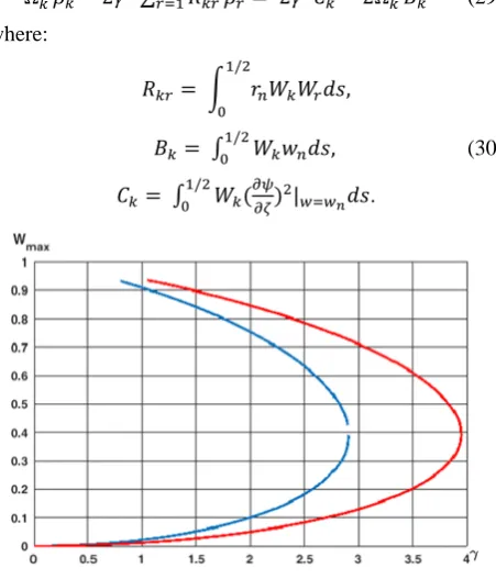
Figure 5. The results of calculation by iteration method (𝜀= 0.1)

Having solved system (29), i.e. determine unknown coefficients 𝛽_𝑘 from system (29) and consequently ∆_𝑛 we can find next approximation: 𝑤_𝑛+1= 𝑤_𝑛+ ∆_𝑛.

The dependence 𝑤_𝑚𝑎𝑥from value of parameter 𝛾 for case then 𝜀𝛼= 0.1 ; 0.2. (with account edge effect) is shown in Fig.5. The dependence 𝑤=𝑤(𝑠) at 𝜀= 0.1,

𝛾= 1.5 on left part of beam is shown in Fig 6. Calculation fulfilled retaining twelve symmetric modes

The inner curve corresponds to the case then𝛼= 1, external for 𝛼= 2. So the increasing of the beam stiffness leads to shift of branching curve to the right

Figure 6. The form of the half of beam under the action of electric force

For solution task without edge effect it’s enough in expression (19) for 𝜕𝜓

𝜕𝜁 take 𝑆= 0, i.e. to solve equation: 𝜀𝛼𝑤𝐼𝑉_{− 𝑤}′′₌_𝛾2 1

(1−𝑤)2 (31)

Comparing the solution of this equation with previous calculation are shown that taking in account the edge effect in our models practically not influence on the branching diagram (for example in Fig.5).

The task of flexure of tensile string (layer) under action of electrostatic force without taking in account first item in eq. (31) yields to analytic solution. In this case the boundary problem takes a form:

𝑤′′₊_𝛾2 1

(1− 𝑤)2= 0,

𝑤(0) =𝑤(1) = 0. (32) The solution of this task taking in account the condition of symmetry relatively middle of string 𝑤′(1 2⁄ ) = 0 leads to integral relation

1

2(𝑤′)2+ 𝛾2

1−𝑤= 𝐶, (33)

where the constant 𝐶 is determined from condition of symmetry as 𝐶= 𝛾2

1−𝑤𝑚, 𝑤𝑚– flexure in a middle of the

string. Using boundary conditions leads to equation relatively 𝑤_𝑚

∫𝑤𝑚�_𝑤1−𝑤_𝑚_−𝑤𝑑𝑤=𝛾�₂₍_1−𝑤1 _𝑚₎.

[image:4.595.62.288.477.741.2]

(5)

In result we obtain the algebraic equation

�𝑤𝑚+ (1− 𝑤𝑚) 𝑙𝑛�₁₋1+_�𝑤�𝑤𝑚_𝑚 = 𝛾�₂₍_1−𝑤1 _𝑚₎ (35)

This equation can be rewrite in form:

𝛾=�2(1− 𝑤𝑚) �𝑤𝑚+√2 ∙(1− 𝑤𝑚)3/2𝑙𝑛�1+₁₋�𝑤_�𝑤𝑚_𝑚

(36) In result the dependence 𝑤_𝑚(𝛾) (36) is shown in Fig.7

Figure 7. Analytic diagram of string branching

With increasing of parameter 𝛾 from zero until point of branching this equation has two solutions. The point of branching corresponds to tangency solution of (36) in point

𝑤𝑚~0.4, that has place at 𝛾∗~1.2. After point of

bifurcation this equation has not solution. It is evidently that at 𝛾<𝛾_∗ the solution with smaller amplitude of flexure is stable in contrast to unstable for of curve with bigger amplitude, both take place at the same value of electric potential.

4. Conclusions

The main achievement of this work is an investigation of the influence of the ratio between flexural and membrane stiffness of micro layer situated in electrostatic field on the point of pull-in effect. Moreover we suppose that the bending stiffness is much less than the stiffness of string. This assumption gives us the possibility to build the asymptotic approximation of pull-in branching curve.

Acknowledgements

The study was carried out by support of grant RFBR RAS 17-01-00414.

REFERENCES

[1] Grinberg Ya.S., Pashkin Yu.Ya. and Ilychev E.V. Nanomechanical resonators//Achievement of Physical science, 2912 – 4: V. 18, pp. 407 – 436.

[2] Wen-Ming Zhang, Han Yan, Zhi-Ke Peng, Guang Meng Electrostatic pull-in instability in MEMS/NEMS: A review // Sensors and Actuators A: Physical, 2014 Elsevier, pp.188-218

[3] John A. Pelesko and Tobin A. DriscollThe effect of the small-aspect-ratio approximation on canonical electrostatic MEMS models// Journal of Engineering Mathematics, 2006, V.53, pp. 239 - 252

[4] Slava Krylov [et al.] Symmetry breaking in an initially curved pre-stressed micro beam loaded by a distributed electrostatic force// International Journal of Solids and Structures, 51, 2014

[5] Bom K. [et al.] Nanomechanical resonators and their applications in biological/chemical detection: Nanomechanics principles // Physics Reports. 2011, V. 503, pp. 115 – 163

[6] Scott Bunch J. [et al.] Electromehanical Resonators from Graphene Sheets // 2007, V. 315, pp. 490 –493

[7] Lior Medina S. [et al.] Large-Scale Arrays of Single-Layer Graphene Resonators // Nano Letters. 2010, V.10, pp. 4869 – 4873.

[8] C. Lee, X. Wei, J. W. Kysar и J. Hone Measurement of the Elastic Properties and Intrinsic Strength of Monolayer Graphene// Science, V. 321, № 5887, pp. 385-388, 2010.

[9] Firsova N.E., Firsov Y.A. A new loss mechanism in graphene nanoresonators due to the synthetic electric fields caused by inherent out-of-plane membrane corrugations// J.Phys.D: Appl. Phys.,V.45, p., 2012.