SRC RR 77 pdf

Automatic Reconfiguration in Autonet

September 18, 1991

SRC Research Report 77

This report is an expanded version of a paper that has been accepted for presentation at the ACM Symposium on Operating Systems Principles, October 13-16, 1991.

 Digital Equipment Corporation 1990.

This work may not be copied or reproduced in whole or in part for any commercial purpose. Permission to copy in whole or in part without any payment of fee is granted for nonprofit, educational, and research purposes provided that all such whole or partial copies include the following: a notice that such copying is by permission of the Systems Research Center of Digital Equipment Corporation in Palo Alto, California; an acknowledgement of the authors and

ABSTRACT

1 . Introduction

Autonet is a switch-based local area network. In an Autonet, 12-by-12 crossbar switches are interconnected to other switches and to host controllers with 100 Mbit/s full-duplex links in an arbitrary pattern. In normal operation each packet follows a precomputed link-to-link path from source to destination. At each switch, hard-ware uses the destination address in each packet as the lookup index in a forwarding table to determine the proper outgoing link for the next step in the path. An earlier paper [15] provides an overview of the Autonet design. In the present paper we concentrate on automatic reconfiguration in Autonet.

Automatic operation and high availability are important objec-tives for Autonet. Our goal was to make Autonet look to host com-munications software like a fast, high-capacity Ethernet segment that never failed permanently. To provide automatic operation and high availability an Autonet automatically reconfigures itself to use the available topology of switches and links. A processor in each switch monitors the directly connected links and neighboring switches. Whenever this monitor notices a change in what is working (either additions or removals), it triggers a distributed algorithm on all switch processors that determines and distributes the new network topology to all switches. Once each switch knows the new topology, it recalculates routing information and reloads its forwarding table to permit operation with the new topology. This automatic recon-figuration is fast enough that high-level communication protocols are not permanently disrupted, even though client packets may be lost while reconfiguration is in process.

When an Autonet is installed with a redundant topology, au-tomatic reconfiguration allows it to continue to provide full interconnection of all hosts as components fail or are removed from service. If there are so many failures that connectivity is lost, the Autonet will partition, but service will continue within each connected portion. When components are repaired, or the topology is extended with new switches or links, automatic reconfiguration incorporates the added components in the operational network.

100 hosts. Operational experience has allowed (forced) us to improve the sensitivity, stability, and performance of the automatic reconfiguration mechanisms. So this paper, in addition to giving a more detailed description than we have previously published on reconfiguration in Autonet, also highlights the important changes that were dictated by our experience.

The paper is organized as follows. Section 2 compares Autonet with other networks with automatic reconfiguration. Section 3 gives the overall structure of reconfiguration in Autonet. Section 4 discusses monitoring and Section 5 topology acquisition. Section 6 presents conclusions.

2 . Reconfiguration in Other Networks

The standard example of automatic reconfiguration in a com-puter network is the ARPANET [10, 11]. The principle differences between ARPANET and Autonet relate to the fact that ARPANET is designed as a wide-area, moderate-speed network while Autonet is designed as a local-area, high-speed network.

The ARPANET performs store-and-forward routing based on topology descriptions maintained at each switch (IMP), and tolerates temporary forwarding loops by discarding packets if necessary. Each switch regularly broadcasts updates of the status of its local links.

The Autonet switch hardware processes packets first-come-first-served from each link and uses cut-through to decrease the ex-pected delay through the switch. This design was chosen because it provided the best light-load performance for the simplest hardware. However as a consequence, transient forwarding loops might result in deadlock and thus cannot be tolerated. We do not have efficient means of detecting a deadlock or of clearing one. We took the sim-plest approach of rapidly recalculating the entire topology whenever it changes and expunging all old forwarding tables before installing any new ones. This global-recalculation design is simpler than in-cremental approaches and represents an appropriate engineering tradeoff for a moderate-sized network of several dozen switches.

updates. PARIS is designed more as a fast connection network than a packet switching network. Packets travel on explicit source routes which are determined at connection setup by examining a description of the current topology. Topology changes have no effect on exist-ing connections, except that a link failure kills all of the connections using that link. Link updates are distributed reliably and with very high bandwidth by hardware flooding over a spanning tree managed by the software. The software tree management is very careful not to introduce inconsistencies into the tree. In contrast to PARIS, Au-tonet routes each new packet independently and thus automatically maintains ongoing conversations by routing around link failures and exploiting link recoveries.

Bridged Ethernet [13] is another network that provides auto-matic reconfiguration. The principle difference from Autonet is that a bridged Ethernet supports multiple-access links with no way to dis-tinguish forwarded packets from originals. A bridged Ethernet carefully maintains a loop-free forwarding tree so that each bridge can deduce what to do with each packet. Although the time constants required to maintain consistency in the forwarding tree are on the order of several seconds, a bridged Ethernet does eventually adapt to any topology change. In contrast, Autonet has an implicit addressing structure induced by its point-to-point links. An arriving packet is al-ways known to be intended for the recipient, at least as an inter-mediate hop. We also designed a packet encapsulation using net-work-assigned destination addresses, in order to make forwarding easier (much like Cypress [4]). As a consequence, Autonet uses more forwarding paths and reconfigures much faster than a bridged Eth-ernet.

3 . The Structure of the Automatic Reconfiguration Mechanism

Monitoring determines which links are useful for carrying client packets from one switch to another. From the point of view of reconfiguration, a link is useful if and only if it has an acceptable er-ror rate in both directions, the nodes at each end are distinct, opera-tional switches, and each switch knows the identity of the other. (A switch is identified by a 48-bit unique identifier stored in a ROM.) Topology acquisition and route recalculation is triggered whenever the set of useful links changes. Of course, host-to-switch links also carry client packets, but changes in the state of such links never trig-ger topology acquisition and route recalculations. At most, changes in the host links to a particular switch cause locally calculated changes in that switch’s forwarding table. So, from the point of view of network reconfiguration, we largely ignore such links.

Monitoring guarantees that topology acquisition (and client) packets will not travel over a link unless both switches agree the link is useful. Because there are two switches involved there will always be transient disagreement whenever the link is changing state, but the monitoring task makes the period of disagreement as brief as pos-sible. A monitor runs independently for each link in each switch and is always active. It will trigger topology acquisition whenever its link changes from useful to not useful or vice versa. The monitors guarantee that, eventually, links remain stable in one state or the other long enough that topology acquisition and routing can finish.

Topology acquisition is responsible for discovering the network topology and delivering a description of it to every switch that is currently part of the network. This task runs in an artificial environment in which changes in link state do not occur. When two switches disagree about the state of a link, the task does not complete. The artificial environment is implemented on top of the monitoring layer by means of an epoch mechanism: any change or inconsistency triggers a new epoch corresponding to a new stable environment. Topology acquisition is a distributed computation that spreads to all switches from the one where a link monitor triggered it.

acquisition and routing, the switch discards client packets. Once the forwarding table has been recalculated, a switch is able to forward any client packets it receives. The reason for discarding client packets during reconfiguration is to prevent deadlock.

The remainder of the paper concentrates on monitoring and topology acquisition. In considering these topics in more detail we can model the Autonet as a collection of nodes (switches) with num-bered ports. Nodes may be interconnected in an arbitrary pattern by full-duplex, port-to-port links. Each node is a computer that can send and receive packets on each attached link that works. Each node has a predetermined unique identifier. From now on we will largely ignore links to hosts, the hosts themselves, forwarding of host packets, and even the forwarding tables in the switches.

The neighborhood of a node N is the set of all useful switch-to-switch links that have N as one endpoint. The neighborhood of a set of nodes is the union of the neighborhoods of the members. Au-tonet reconfiguration can be characterized in terms of these neighborhoods. The monitoring task on node N is responsible for knowing the current neighborhood of N, and for initiating a topol-ogy task whenever the neighborhood changes. Topoltopol-ogy acquisition works by building a spanning tree, merging neighborhoods of larger and larger subtrees until the root has the neighborhood of the entire graph, and then flooding the topology down the spanning tree to all nodes.

We are now ready to describe monitoring and topology acquisition in more detail. In this discussion, “packet” and “signal” refer to information passing between separate nodes over a con-necting link. Packets are regular data packets whereas signals are transported in link protocols below the level of packet traffic. “Mes-sage”refers to information passing between software components in a single node.

4 . Monitoring

change. For example, if a technician powers off a switch, all of the adjacent nodes see link failures on their links to the dead node.

The monitoring task responds rapidly to link failures and less rapidly to link recoveries. Link failure, especially abrupt failure, must be detected and reported quickly, because failure can disrupt ongoing client communication. It is not so urgent to rush back into service a link that recently gave problems. Although it is true that link recovery might heal a network partition or increase network ca-pacity, repairing or adding a link usually takes quite a bit of time, so clients usually will not notice a small additional delay. Many net-works, for example, the ARPANET, have a delay before placing links back in service [7]. By delaying longer as a link proves its unreliability, we achieve network stability despite intermittent failures.

A useful link is one that allows bidirectional packet transfer with acceptably low error rates between two distinct nodes. The only way this condition can be verified, of course, is for the two nodes to periodically exchange packets, and this is what the monitoring task does. This strategy has the advantage that it is an end-to-end check [14]. It has the disadvantage that failure detection may not be very prompt, because it depends on a timeout whose minimum value is bounded by processing overhead. In order to give prompt detection of expected modes of link failure, the monitoring task also treats certain kinds of hardware errors as indicating failure. For example, if more than three link coding violations are detected in a ten-millisecond interval, the monitoring task immediately as-sumes that the link has failed.

4.1. The Skeptic

The skeptic limits the failure rate of a link by delaying its re-covery if it has a bad history. Without the skeptic, an intermittent link could cause an unlimited amount of disruption: we are espe-cially concerned with limiting the frequency of reconfigurations. There are four requirements in the design of the skeptic: 1) A link with a good history must be allowed to fail and recover several times without significant penalty. 2) In the worst case, a link’s average long-term failure rate must not be allowed to exceed some low rate. 3) Common behaviors shown by bad links should result in exceed-ingly low average long-term failure rates. 4) A link that stops being bad must eventually be forgiven its bad history.

Requirement 3 distinguishes the skeptic from typical fault iso-lation and forgiveness methods such as the autorestart mechanism in Hydra [17]. The typical method to meet requirements 1, 2, and 4 sets a quota of say, ten failures per hour, and refuses to recover any link that is over quota. We have observed a common pattern of in-termittent behavior in which a link fails again soon after being recovered, in spite of its passing all diagnostics performed in the in-terim. With the quota method, this pattern would produce a long-term average failure rate of ten failures per hour. This kind of error pattern may not be uncommon, for example Lin and Siewiorek observed a clustering pattern of transient errors in the VICE file system [9].

The skeptic can be used with any object whose status may change intermittently: it provides a “filtered object” whose rate of status change is limited. As seen by the skeptic, an object is an ab-straction that emits a series of messages, each of which says either “working” or “broken”. The skeptic in turn sends out a filtered ver-sion of these messages to the next higher level of abstraction. This operation is shown in Figure 1.

4.1.1. Details of the skeptic

that information, and good state means that the object is working and the skeptic has concurred.

“broken” “working”

skeptic

“broken” “working” subordinate

object

filtered object

Figure 1: The concept of the skeptic.

dead good

wait

recv “broken”

recv “broken”

recv “working”

wait timer expires send “broken”

send “working”

–1 level +1 level

skepticism level

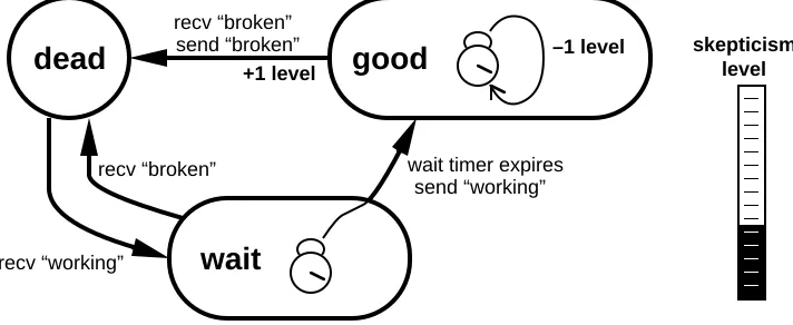
Figure 2: The internals of the skeptic.

When the skeptic moves from wait to good, it sends a “working” message to the next higher level of abstraction. When the skeptic moves from good to dead, it sends a “broken” message. Hence, in the filtered view provided by the skeptic, the object appears to be working only when the skeptic is in good. If the subordinate object fails intermittently, the skeptic alternates between dead and wait without ever reaching good.

When the skeptic enters wait state, it sets and starts the wait timer. The duration set on this timer is calculated by a formula de-scribed below. If the skeptic returns to dead before the timer ex-pires, the timer is stopped. Otherwise, when the timer exex-pires, the skeptic moves to good. This is the only way the skeptic can get to good state.

The skeptic responds to intermittent failures by maintaining a level of skepticism about the subordinate object. The skepticism level is kept in an auxiliary variable. Every time the skeptic leaves good state it increments the level. The skepticism level is used in computing wtime, the duration set on the wait timer, according to the formula

wtime = wbase + wmult * 2level

where wbase and wmult are policy parameters and level is the skepticism level. A policy parameter maxlevel establishes an upper limit on skepticism.

The skeptic forgives old failures by decrementing the skepti-cism level occasionally. When the skeptic enters good state, it sets and starts the good timer. When the good timer expires, the skeptic decrements the skepticism level and sets and starts the good timer again. The good timer is always running as long as the skeptic is in good state. When the skeptic leaves good state, the good timer is stopped. The formula used to compute gtime, the duration set on the good timer, is identical to the formula used for the wait timer, except that it uses different policy parameters, gbase and gmult. The skepticism level never decrements below zero.

monitor, shown in Figure 3. The fault monitor relays the state of the subordinate object to the skeptic. Whenever the fault monitor re-ceives a “fault” message and the subordinate object is working, the fault monitor presents an interruption to the skeptic by sending it “broken” immediately followed by “working”. This causes the skeptic to notice the fault and enter wait state. If the subordinate object was already broken, the fault monitor takes no action on a “fault” message.

fault monitor

“broken” “working”

“broken” “working”

skeptic

“fault”

Figure 3: The skeptic with the fault monitor.

In the actual implementation, the fault monitor and the skeptic are combined together as one unit. Procedure calls are used for the messages.

There is one more feature in the skeptic, which is that the du-ration set on the wait timer actually varies as a random fraction be-tween one and two times the value calculated for wtime. This ran-dom variation causes different skeptics to disperse their wait-timer expirations. If the network is running with several intermittent links, this randomness reduces the possibility of getting caught in some systematic pattern.

4.1.2. How the skeptic works in practice

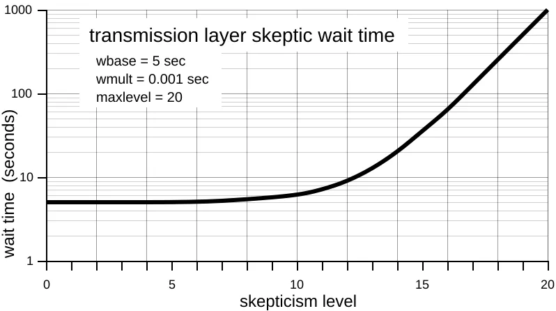
Figure 4 shows an example of how the skeptic wait timer be-haves, using the policy parameters of the transmission layer. Ob-serve that at low skepticism levels, the wait time is dominated by

wbase, which is constant, whereas at high levels, the wait time is

The crossover between low and high levels occurs when the two terms are equal:

crossover level = log2( wbase / wmult )

The transmission layer skeptic crosses over at about level 12. Policy parameters for our skeptics are given in Table 1.

skepticism level

0 5 10 15 20

1000

100

10

1

wait time (seconds)

transmission layer skeptic wait time

wbase = 5 sec wmult = 0.001 sec maxlevel = 20

Figure 4: Skepticism level versus wait time.

transmission

skeptic connectivityskeptic

wbase wmult gbase gmult maxlevel

5 sec 0.001 sec

600 sec 0.01 sec

20

1 sec 0.1 sec 600 sec

0.1 sec 20

A few examples of how the transmission layer skeptic re-sponds to common problems will illustrate its utility.

One common mode of link failure we have observed, espe-cially in newly installed hardware, is that the link transceiver hardware continuously detects coding violations. In this case, the transmission layer will declare a fault about once every 170 millisec-onds. Because this is much less than the five-second minimum wait time, the skeptic never lets the link recover. To higher levels of ab-straction, the link appears permanently broken.

Another common failure mode occurs when a technician screws in a link cable. As the metal components scrape past each other, the link transceiver hardware detects bursts of coding viola-tions that the transmission layer quite reliably evaluates as faults. Unfortunately, the cable connectors we use are quite difficult to thread correctly, and often several tries and some wiggling are needed before the cable allows itself to be properly screwed in. Each additional wiggle tends to generate more faults. The five-second minimum wait time in the skeptic causes all of these faults to be reflected as only one failure.

A third common failure mode occurs on marginal links. In our experience, the error rate on a marginal link is very data depen-dent: it is much higher when the link is carrying packets than when it is idle. This results in such a link failing soon after it recovers, but then having no further faults until it recovers again. The skepti-cism level on such a link increases over time. Eventually the skepticism level in the transmission layer reaches its maximum value of 20, at which point the wait time is about 17 minutes. If the link is part of the switch-to-switch topology, so that failures and recoveries cause network-wide reconfigurations, the connectivity layer skeptic gets involved, and its policy parameters produce a maximum wait time of about 28 hours.

4.1.3. Fulfillment of our design requirements

Now let us consider how the skeptic fulfills our design re-quirements.

1) A link with a good history must be allowed to fail and recover several times without significant penalty. We interpret

Rapid cycles of failure and recovery in the subordinate object increase the skepticism level by one each cycle, but at low skepticism levels, the skeptic’s delay in wait state is dominated by the constant

wbase, which is chosen to have a small value of only a few seconds.

Consequently, during the first several cycles of failure and recovery, the filtered object recovers soon after the subordinate object recov-ers.

2) In the worst case, a link’s average long-term failure rate must not be allowed to exceed some low rate. The worst case

long-term average failure rate of the filtered object occurs when the skep-tic spends the minimum time in good state required to forgive the lowest level of skepticism. This minimum time is slightly larger than gbase and hence the long-term average failure rate cannot ex-ceed 1/gbase. A sketch of the proof is as follows. Each failure of the filtered object creates a level of skepticism. It takes at least

gbase time in good state to forgive a level of skepticism, so we

count each gbase interval in good state as an opportunity to “forgive” a failure. At a sufficiently high level of skepticism, say N, the wait time is at least gbase. We count each gbase interval in wait state as an opportunity to “forget” a failure. Each level of skepticism from 0 to N-1 we count as an opportunity to “retain” a failure. Now over a period of time each failure must be counted under one or more of these opportunities. Therefore over a period of time t there can be at most (t/gbase)+N failures. We assume N does not exceed maxlevel.

3) Common behaviors shown by bad links should result in ex-ceedingly low average long-term failure rates. The interesting

be-havior here is when the subordinate object tends to fail again soon after the filtered object has recovered. If the failure happens before the good timer expires, then the skepticism level increases over time. At sufficiently high skepticism levels, the wait time becomes significant and increases the interval between failures by delaying the recovery of the filtered object.

4) A link that stops being bad must eventually be forgiven its bad history. If the subordinate object remains working for a long

4.1.4. Choice of skeptic parameters

We chose the skeptic parameters as follows. The transmission layer skeptic deals with physical phenomena, so several of its pa-rameters derive from maintenance needs. Five seconds is the short-est minimum wait time that will cover the process of screwing in a link cable. A technician often recables a host controller several times during testing, so we allow about eight levels before the in-crease in wait time becomes perceptible. Twenty minutes is the longest time a technician will bear before seeing whether an at-tempted hardware repair has any effect on the system. Ten minutes seems like a reasonable interval for the minimum good time.

We expect problems in the connectivity layer to be unusual ex-cept when induced by the transmission layer, so we set its minimum wait time smaller, at one second, and its crossover point lower, at level four. Because failures in the connectivity layer cause network-wide reconfigurations, the maximum wait time should be as long as possible. We chose 28 hours because we did not want the system to hold off much more than a day on its own authority.

4.1.5. Relation to other work

Many networks contain a mechanism for discriminating against unreliable links. For example, PARIS [2] increments a reli-ability counter with each link failure. (The value of this “relireli-ability” counter actually represents unreliability.) The current value of a link’s reliability counter forms the most significant component of a link’s weight, which is broadcast regularly in updates of the link sta-tus. Connection setup and the tree manager shy away from links with high weight, and thus unreliable links will tend not to get used unless necessary. The value in a link’s reliability counter decays over time so that information about old failures expires eventually [1]. However, PARIS does not have a backoff strategy, so if the unreliable link is the only connection between two parts of the net-work, PARIS will suffer repeated topology changes rather than permit the network to remain partitioned.

speculation supports the exponential increase in wait time at high skepticism levels.

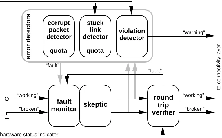
4.2. The Transmission Layer

The transmission layer contains a skeptic with a fault monitor, three error detectors, and a round trip verifier, shown in Figure 5. The transmission layer watches the error indicators in the link hard-ware and determines if the link appears to be successful at sending and receiving data. It passes its conclusion up to the connectivity layer. The transmission layer does not care where the data might be going to or coming from—it is the responsibility of the connectivity layer to determine that. If the transmission layer determines that the link is broken, it sets the switch hardware to discard all incoming and outgoing packets, isolating the link. No packets can be sent or received over an isolated link. The reason for isolating a broken link is to prevent it from interfering with the rest of the network.

fault monitor

“broken” “working”

“broken” “working”

skeptic

“fault”

round trip verifier

violation detector hardware status indicators

“warning” stuck

link detector

“fault”

quota corrupt

packet detector

quota

hardware status indicator

error detectors

to connectivity layer

The fault monitor here at the lowest level of the system really has no subordinate object, so it is connected to a dummy object that is always working. “Working” and “broken” are abstractions that are synthesized based on the hardware status indicators, as interpreted by the error detectors and round trip verifier. The round trip verifier filters the output of the skeptic by delaying “working” messages until it believes that the transmission layer skeptic on the other end of the link also believes the link is working.

Each of the three error detectors analyzes and responds to a different type of error indicated in the switch hardware.

4.2.1. The corrupt packet detector

The corrupt packet detector examines all packets received by the switch control processor and declares a fault when CRC errors or impermissible packet lengths are seen too frequently. It is possi-ble for packets to be corrupted without any detectapossi-ble coding viola-tions, when a data error happens inside the crossbar at some switch. Such an error is eventually detected as a CRC error at the packet’s ultimate destination. It would be better if each link verified the CRC of all incoming packets, but this feature was omitted from the hard-ware. We achieve some protection against corruption by checking all of the packets destined for the local switch control processor.

An isolated corrupt packet might be the result of a random glitch, so it should be forgiven. Corrupt packets become a significant error if they happen too frequently. The corrupt packet detector imposes a quota on how often it forgives corrupt packets by using a leaky bucket mechanism [16]. Every time it encounters a corrupt packet, it puts a token in the bucket. One token leaks out of the bucket every ten minutes. Whenever adding a token to the bucket causes the bucket to hold more than five tokens, the corrupt packet detector declares a fault. Because the transmission layer isolates a broken link so that it can neither send nor receive packets, no further corrupt packets will arrive from the link until the skeptic recovers it.

4.2.2. The stuck link detector

some corruption of flow control commands. If a link has been trying to transmit a packet, but has made no progress for several milliseconds, something is wrong on the link. At this point it is necessary to dump the stuck packet and free up its resources.

This recovery is bound to be disruptive, although in our switches it is perhaps more disruptive than absolutely necessary, since our only mechanism for dumping a packet is to reinitialize the entire switch. This destroys all packets in the switch. Fortunately, reinitializing only takes about ten microseconds. Isolating a broken link removes the opportunity for it to cause further switch reinitial-izations.

Although a stuck link should not happen in normal operation, links can appear to be stuck as a result of mistransmission of a single command code pertaining to flow-control or packet framing. Thus the stuck link detector must be willing to forgive an isolated oc-currence. The detector samples its hardware indicators every 100 milliseconds and, if the link is stuck, responds by reinitializing the switch. The stuck link detector imposes a quota on how often it for-gives by using a leaky bucket mechanism to declare faults, exactly like the corrupt packet detector.

4.2.3. The violation detector

The violation detector analyzes and responds to coding and format violations received on the link. A coding violation basically means that the link receiver heard a piece of static on the line. For example, coding violations result from connecting or disconnecting the link cable, from a cable that is too long for good transmission, or from a nearby heavy-duty electric motor. Although connecting or disconnecting a link generates a burst of coding violations tens of milliseconds long, even the best links in our system pick up one or two isolated coding violations per week. A format violation means that the link receiver did not hear proper packet framing or flow-control where it expected. Static can cause isolated format viola-tions, as can occasional activity such as reinitializing the switch. Hence a burst of violations is a significant error, but isolated viola-tions should be ignored.

block of 128 samples. At the end of each block, the violation de-tector checks the number of violations and, if there are too many it declares a fault. The permitted number of violations depends on whether the skeptic says the link is working or broken, which is why Figure 5 shows the error detectors receiving the “working” and “broken” messages from the skeptic. If the link is working, three er-rors are permitted in a block, but if the link is broken no erer-rors are permitted. The more strict rule for broken links insures that no link will recover unless it can pass the entire skeptic recovery time with-out a single violation, while occasional violations on working links are ignored.

If a broken link continues to have violations, the violation de-tector continues to declare a fault at the end of each block. The transmission layer skeptic always spends at least five seconds in wait state, so it will keep believing that the link is broken.

In order to detect promptly the bursts of violations that result from the anticipated activity of plugging and unplugging link cables, the violation detector examines subblocks of eight samples. If a sub-block contains more than three violations, the violation detector im-mediately declares a fault. In order to eliminate the processing over-head of declaring faults every subblock, subblock checking applies only to working links.

Our method of ignoring occasional problems by declaring a fault only when more than three violations occur in 128 samples is known as the k out of n method. This method is used in testing neighbor reachability in the Internet’s Exterior Gateway Protocol (EGP) [12] and in the Cypress network [4]. For simplicity, we test k out of n only at the end of n samples, rather than continuously. EGP also shares our idea of using different threshold parameters depend-ing on the current state of the link.

4.2.4. The round trip verifier

working, then it declares the link to be working. Otherwise, the link is broken. This function is implemented by the round trip verifier.

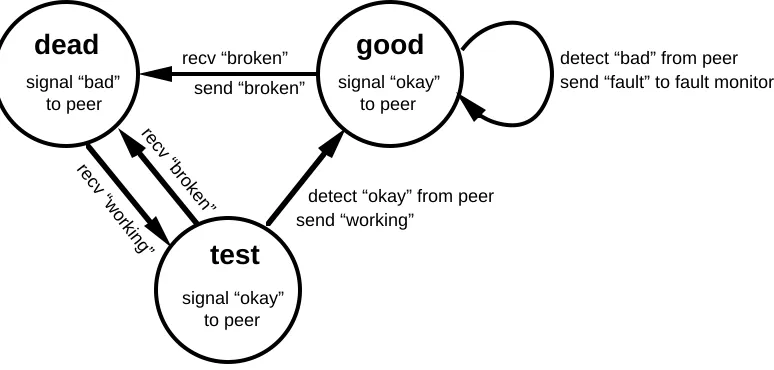
The round trip verifier contains a state machine with three states: dead, test, and good, shown in Figure 6. Because it supports the same structure of interactions between subordinate object and fil-tered object as the skeptic, the state machine resembles that of the skeptic (Figure 2). Dead state means that the underlying skeptic de-clares that the link is broken, test state that the skeptic dede-clares the link is working but the remote node does not yet concur, and good state that both agree the link is working.

dead good

test

recv “broken”

recv “working” recv “broken”

send “broken”

send “working”

detect “okay” from peer signal “bad”

to peer

signal “okay” to peer

signal “okay” to peer

send “fault” to fault monitor detect “bad” from peer

Figure 6: Round trip verifier state machine.

The round trip verifier uses the flow-control channel on a link to send a signal to the other node. The flow-control channel is a dedicated time slot in which the link’s transmitter normally sends flow-control command codes. Under software control, the transmitter fills this slot instead with a distinguished command code called idhy, which stands for “I Don’t Hear You”. The round trip verifier uses idhy to send a “bad” signal, and uses the absence of

idhy to send an “okay” signal. The verifier receives these signals by

The round trip verifier continually sends “bad” to its peer in dead state and “okay”in test state and good state. Because the link transports these signals below the level of packet traffic, the nodes can exchange this information even when the link is isolated. The verifier remains in test state until it detects an “okay” signal, at which point it moves to good. When the verifier is in good state, it immediately declares a fault if it ever detects a “bad” signal. The fault causes the underlying skeptic to declare the link broken which results in the verifier moving back to dead state. The verifier sends and receives “working” and “broken” messages from adjacent software layers just like the skeptic does.

Notice the effect of the round trip verifier on a link that works well in only one direction, say from node A to node B. The error detector in node B has no cause for complaint and its skeptic declares that the link is working. The error detector in node A is upset and its skeptic declares that the link is broken. The round trip verifier in node A is signalling “bad”, which tells the round trip verifier in node B that A is upset. Consequently, the transmission layers in both nodes agree that the link is broken. The verifier in A is in dead state and the verifier in B is in test state.

Now suppose that the link is repaired and the error detector in node A is now happy. After the skeptic recovery delay, the round trip verifier in node A moves to test state and begins signalling “okay”. It detects “okay” from B, which is in test state, and moves to good state. The round trip verifier in node B soon detects the “okay” from A and moves to good state. Both nodes now believe that the link is working. The transmission layer always brings a link up with this handshake.

link is taken out of isolation so that packets can pass across it to the host.

As we have seen, the transmission layer filters out links with error conditions and links that connect to host controllers. It is the job of the connectivity layer to filter out links that do not connect anywhere or that connect back to the same switch.

4.3. The Connectivity Layer

The connectivity layer comes into action once the transmission layer has declared that a link is working. The connectivity layer sends packets back and forth across the link to determine if the link is a useful noto-node connection. When the connectivity layer de-clares that a link is useful, it also provides the identity of the remote node. The union of the results of the connectivity layers for the links at a node comprises the current state of the neighborhood monitoring task at that node.

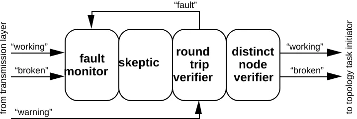
The connectivity layer contains a skeptic with a fault monitor, a round trip verifier, and a distinct node verifier, as in Figure 7. The fault monitor receives the messages from the transmission layer about whether the link is working or broken. The round trip verifier filters the output of the skeptic by delaying “working” mes-sages until it has exchanged packets over the link and has determined the identity of the remote node. The distinct node verifier filters the output of the round trip verifier by checking that the remote node is indeed different from the local node. Whenever the connectivity layer generates either a “working” or “broken” message, topology acquisition is initiated.

fault monitor

“broken” “working”

“broken” “working”

skeptic

“fault”

round trip verifier

from transmission layer

distinct node verifier

“warning” to topology task initiator

Figure 7: Diagram of the connectivity layer.

The round trip verifier exchanges connectivity packets with its peer on the remote end of the link, to determine the identity of its peer. Peer identity (id) has two components: a 48-bit unique node identifier and a 4-bit port number within the node. To insure that an identity is current, we create a sequenced identity (s-id) by attaching a 32-bit sequence number. The round trip verifier knows its own lo-cal s-id and it maintains a current estimate of the s-id of its remote peer. A connectivity packet carries the local and remote s-ids from the transmitter as source and destination s-ids.

The connectivity round trip verifier has a state machine simi-lar to that of the transmission round trip verifier. In place of detect-ing “okay” and “bad” signals, the connectivity round trip verifier checks the result of a round trip exchange of connectivity packets.

Some connectivity packets are requests and others are replies. The only difference is that the receiver must send back a connectivity packet in response to a request, whereas a reply does not need a re-sponse. Requests and replies are distinguished by a flag in the packet header.

first but backs off exponentially if no matching packet is forthcom-ing.

The round trip verifier continues sending request packets in good state, and it expects confirming packets to be received. A con-firming packet contains a destination s-id equal to the local s-id and a source id equal to the remote id. (It is not necessary to inspect the remote sequence number to insure that the packet exchange is cur-rent.) We save the source s-id as the estimate of the remote s-id and increment the local sequence number. A packet that would be con-firming except that the destination and local sequence numbers fail to match is ignored. Any other received connectivity packet causes an immediate fault (which, in turn, causes the skeptic to declare the link broken and the verifier to move to dead state). The verifier transmits requests very frequently at first but backs off exponentially as confirming packets are received. When confirming packets fail to be received within five times the transmission interval, the interval is decreased by half and another five transmissions attempted. A fault is declared if the interval had already attained its minimum value.

Whenever the skeptic declares that the link is broken, the round trip verifier passes on the declaration and enters dead state. In dead state, the round trip verifier sends no requests. If any requests are received during dead state, they are answered with replies that good state treats as contradictory and test state ignores.

The effect of the round trip verifier is as follows. Suppose that the link appears healthy to the transmission layer but connects to a node that does not answer. The round trip verifier will be in test state and will back off exponentially until the transmission rate is one request packet every ten seconds. Now suppose that the remote node begins responding. With the first matching reply, the round trip verifier moves to good state with the minimum transmission interval. As confirmations arrive, the transmission interval increases to its maximum, at which point the round trip verifier will be sending one request packet every ten seconds to continue verifying that the link is still working.

reasonable response time is still provided in the case of complete autism.

The distinct node verifier filters the output of the round trip verifier by comparing the remote node identity against the local node identity. If they are equal, the distinct node verifier does not pass on the declaration that the link is working. Links that connect back to the same node are not useful node-to-node connections even though they may carry packets perfectly. Whenever the distinct node verifier changes a link from “working” to “broken” or back, the neighborhood monitoring task declares a change in the neigh-borhood, which causes the topology task to recompute the network topology. The topology task is discussed in detail later.

In addition to the actions described above, the round trip veri-fier also responds to warnings issued by the error detector in the transmission layer. The error detector issues an immediate warning whenever it detects one or more violations in a subblock, assuming the condition is not serious enough to warrant declaring a fault. The round trip verifier in the connectivity layer responds to a warning in good state by resetting its transmission interval to the minimum. This results in rapid transmission of round trip request packets and a fault if no confirmation is soon received. Warnings are ignored in dead state and test state.

All packets sent by the topology task, to be described in Section 5, have a header that contains the source id. These values are checked against the remote id and any mismatch results in a connec-tivity fault just like receiving a contradictory connecconnec-tivity packet. If the distinct node verifier says that the link is broken, any topology packets received will be discarded.

4.4. Development History and Experience

tended to provoke a lot more errors than links that were being tested. At that time the topology task took about five seconds to complete, so the network was completely unusable. The skeptic fixed the problem by effectively removing marginal links from the network.

We encountered another difficulty due to a malfunctioning host controller that sent incorrect flow control commands. This caused the adjacent node to get stuck when it attempted to send a packet to the host. We had not realized how important it would be to detect stuck links. The stuck node could not respond to connectivity requests from its neighbors, so after ten seconds they gave up and re-configured. The stuck node also reconfigured into a partition by it-self. Part of reconfiguration involves reinitializing the crossbar switch, which has the side effect of unsticking a stuck node. The node would then join back with its neighbors and everyone would re-configure again. Soon the node would attempt to send the host an-other packet, and the process would repeat. Once we implemented the skeptic it defended against this problem by effectively partitioning the stuck node out of the network, which at least saved the network from collapse. Implementing stuck link detection allowed links with specific problems to be identified and isolated, without partitioning the network.

This was unexpected. Users were unhappy. Implementing the warn-ings caused the end-to-end check to detect the failure promptly and fixed the problem.

One excellent success of the connectivity layer occurred when a node’s crossbar switch started acting erratically. The crossbar began switching occasional packets to the wrong output link. The neighboring nodes would detect a connectivity violation and break their links, but the links would then seem to work fine in test state so they would recover for a while before breaking again. Eventually the skeptics partitioned the malfunctioning node out of the network.

One scenario that exercises most mechanisms in the monitor-ing task is the powermonitor-ing-on of a switch. Let A be a switch that is about to be powered-on. As mentioned above, a powered-off switch reflects data perfectly. Therefore, while A is powered-off, all of its neighbors B, C, and D see links that work fine at the transmission layer and at the connectivity layer, except that the distinct node veri-fier refuses to pass on the working declaration. The connectivity layer round trip verifiers are in good state at maximum back-off level. Now a technician powers on A. The software initializes all the state machines in dead state, which causes A’s transmission layer round trip verifiers to send idhy. Switches B, C, and D probably hear enough static during the power-on to declare faults, but if not, then their transmission layer round trip verifiers will do so when the

idhy from A starts arriving. At this point everything pauses at least

5 . Topology Acquisition

The monitoring task provides each node N with a description of its neighborhood. In this description the links that do not work or that connect from N back to N have been eliminated. The responsi-bility of the topology acquisition task is to provide each node with a description of the current topology of the entire network.

We first describe the basic method of the topology task assum-ing a very simple scenario: some sassum-ingle node initiates the task (for an unknown reason) and the task runs to completion without any confusion from topology changes (which are assumed never to hap-pen). Then we describe how to extend the basic method to deal with multiple initiators and with topology changes.

5.1. The Basic Method

Let us consider a single instance of topology acquisition as if it were the only thing that ever happened in the network. The basic method presumes that the network is quiet, some single node sponta-neously initiates the topology task, it runs for a while, and then the network is quiet forever after. Note that, even in this simple case, it is possible that two nodes may disagree about the state of their con-necting link. In this circumstance it is required that the topology task never claim to produce a complete topology description.

The topology acquisition task consists of three phases: 1) prop-agation, which constructs a rooted spanning tree over the set of all reachable nodes; 2) collection, which merges together descriptions of larger and larger subtree neighborhoods; and 3) distribution, which sends the complete description from the root back down the spanning tree to all nodes.

The propagation phase consists of a wave of packets that spreads across all links through the network starting from the initi-ating node. The initiiniti-ating node becomes the root of the spanning tree, and each other node joins the spanning tree by designating as its parent link the link on which it is first contacted. This is called a

propagation order spanning tree. Generally one would expect the

During the propagation phase, each node N in the spanning tree contacts each of its neighbors, M, to offer M the opportunity to join the spanning tree as a child of N. If M has not yet joined the spanning tree, it accepts the offer and joins. M then contacts each of its neighbors, in turn. Otherwise, M is already in the tree, and it re-fuses the offer. M sends back a reply to N so that N knows whether M accepted or refused. In this way each node comes to know its parent and its children in the spanning tree.

During the propagation phase each node conducts a query-re-ply exchange with each of its neighbors. The neighborhood monitoring task guarantees that topology-task packets will pass only if both end nodes agree that the link is useful. Suppose there is disagreement about the state of a link between nodes P and Q: P considers the link to be useful but Q does not. Then the propagation phase will get stuck when it arrives at P, because P will not be able to get a reply from Q. Therefore the propagation phase will manage to finish building a spanning tree only if all nodes agree about the state of their connecting links.

The propagation phase dies out when all nodes have been con-tacted and a spanning tree has been formed. This is a global condi-tion, however, and no individual node knows when it has been at-tained. Instead, there is a rolling transition from the propagation phase to the collection phase that begins at the leaves of the spanning tree. A node knows that it is a leaf in the spanning tree when it has contacted all of its neighbors and they have all refused to be chil-dren.

The collection phase begins at the leaves of the spanning tree and rises up to the root. When a node M accepts a propagation-phase offer to be a child of N, it also commits to sending up to N a descrip-tion of the neighborhood of M’s subtree. If M is a leaf in the spanning tree, this is easy, because the link monitoring task provides each node with a description of its neighborhood. Otherwise, M has children. In this case, M waits for subtree neighborhood descriptions from all of its children, merges them together with the description of its own neighborhood, and then sends the result on up to N.

its neighborhood and descriptions from all of its children and has a description of its subtree neighborhood. But of course, in the case of the root, this is a description of the entire network. At this point the collection phase ends and the distribution phase begins. The root sends to each of its children the full network description. The chil-dren in turn send it to their chilchil-dren, and so on, until every node in the network possesses the full network description.

5.2. Multiple Initiators

The basic method assumes that exactly one node initiates the topology task. Now we extend the method to deal with multiple initiators. Multiple initiators cause confusion because more than one node is claiming to be the root of the spanning tree. The confusion is solved by separating the activity into distinct instances of the topology task based on the initiator. Each initiator creates a new, distinct instance of the topology task, which runs independently of all other instances. All state records and packets are labeled with the unique identifier of the initiator in order to keep things straight.

To make efficient use of time and space, we do not want to run multiple instances of the topology task to completion. Also, the topology task is supposed to come to a single definite conclusion in each node. The solution is to conduct a competition during the propagation phase, so that exactly one instance wins and completes the phase, while all the others die out. Observe that the propagation phase spreads over the entire network, so if multiple instances do get started, they will come into competition with each other. Because the propagation phase has no definite end but instead rolls into the collection phase, no node knows which instance wins the competition until the end of the collection phase.

identi-fier labels of the instances. The instance with the lower unique iden-tifier wins.

With the further proviso that only those nodes that do not yet belong to an instance may initiate instances, this competition assures us that exactly one instance will manage to complete the propagation phase—it will be the instance whose initiator has the lowest unique identifier over all initiators. All other instances will die out, as their nodes get taken over by the winning instance.

5.3. Topology Changes

We have extended the basic method to deal with multiple initiators. Now we further extend the method to deal with topology changes. Topology changes cause confusion because the method de-pends on running in a network whose topology is stable. So we simulate a stable topology by using an epoch mechanism. Each node maintains an epoch number that identifies the epoch in which its topology task is running, and this epoch number is included in all topology task packets. When a node’s neighborhood monitoring task reports a change in the neighborhood, the node forgets all of its old topology task state, increments its epoch number, and initiates a topology task in the new epoch. Whenever a node receives a topol-ogy task packet, it compares the epoch number in the packet to its own epoch number. If the packet has an old epoch number it is ignored, if it has the current epoch number it is processed, and if it has a new epoch number, the node forgets all its old topology task state, adopts the new epoch number, and then processes the packet. In this latter case, the only possible packet is an offer to join the spanning tree.

One way to think of epochs is as competing instances of the topology task. (Of course, these instances may have their own sub-instances created by multiple initiators.) Each node is always trying to promulgate the newest epoch it has heard about. We optimize the competition by having a node keep track of the state of the topology task only for the newest epoch.

epoch number. If any changes occur in the node’s neighborhood, the neighborhood monitoring task reports it and the node advances to the next epoch. If there are nodes with inconsistent neighborhoods, which is a possible transient state of the network, the neighborhood monitoring task rapidly eliminates these inconsistencies and reports neighborhood changes in at least one of the affected nodes, which causes new epochs to be created.

5.4. Development History

An initial version of our terminating distributed spanning tree algorithm was invented in 1987 by Leslie Lamport and K. Mani Chandy. The current topology task method differs principally in constructing a propagation-order spanning tree with the initiator as the root. Lamport and Chandy’s version constructs a unique mini-mum-depth spanning tree with the node of globally lowest unique identification as the root. In fact, we still use the Lamport-Chandy tree as our broadcast distribution tree, but each node computes it from the topology description rather than during reconfiguration. The current method also provides for retransmission and acknowl-edgement to deal with lost packets.

Although experience has not revealed problems with the basic algorithm, considerable work has gone into tuning the implementa-tion. Initially, we had 27 switches in our network, and the goal was reconfiguration in less than 200 milliseconds. The original imple-mentation took about five seconds to run the topology task. Clearly this was unacceptable.

discoveries are described below. Table 2 shows the history of per-formance improvement in the topology task.

time (ms)

next

i m p r o v e m e n t

5000 1. postpone forwarding table calculation

1400 2. reduce propagation timeout from 500ms to 20ms 993 3. delete debugging printout of forwarding table 576 4. convert to propagation order tree

540 5. polish collection and distribution code 538 6. use checksum instead of CRC

439 7. reduce competition of initiators

425 8. implement special distribution method

255 9. reduce collection timeout from 100ms to 30ms 207 10. new packet handling scheme for reduced overhead 183 11. reduce collection timeout from 30ms to 10ms 166 12. delete residual overhead from old packet scheme 154

Table 2: Performance improvement milestones.

We saved about 3600 milliseconds when we discovered that each node was calculating its forwarding table after receiving the new topology description but before sending it on to its children. The calculation took about 700 milliseconds and added a delay to the critical path at each level in the tree. We changed the code to send the topology first and then calculate the forwarding table. This work appears as improvement 1 in Table 2.

order to purge old client traffic, during which time the node is deaf for about 15 milliseconds. If the nodes do not purge old client traffic, forwarding cycles may arise during reconfiguration and cause deadlock or regenerative broadcasts. We tried doing without the purge and sure enough, we occasionally got regenerative broad-casts, which, due to a bug in the host controller microcode, tended to crash the hosts. Because the original switch software for retrans-mission had too much overhead to permit the desired small timer values, we had to reimplement it as part of this improvement. This work appears as improvements 2, 9, 10, 11, and 12 in Table 2.

We saved about 420 milliseconds when we discovered that each node copied its forwarding table into its debugging log. The debugging log is flexible, but very slow. We thought these printings were not on the critical path, but it turned out that some were. The simplest solution was just to delete the printings. This work appears as improvement 3 in Table 2.

We saved about 100 milliseconds when we replaced our soft-ware CRC algorithm with a softsoft-ware checksum for topology packets. There is no hardware support in the switches for CRC, so it had to be performed in software. The software CRC algorithm requires 3.32 microseconds per byte, whereas the software checksum requires only 0.42 microseconds per byte. This work appears as improvement 6 in Table 2.

At this point we saw that the majority of the run time went into the topology distribution phase. We completely reimplemented this phase and saved about 170 milliseconds. The original implemen-tation unmarshalled the topology description packets into an internal data structure and then for each child remarshalled the data structure back into packets to send. The redesigned implementation marshalls the data structure once at the root, distributes the packets from parent to children as quickly as possible, and then unmarshalls the data structure in all nodes in parallel. This work appears as im-provement 8 in Table 2.

26 milliseconds. A later simplification saved an additional 14 milliseconds. Polishing all the code in the collection and distribution phases saved a total of 2 milliseconds. Changes guided by the performance trace were much more effective at speeding things up.

The final result of performance tuning was a system that ran the topology task in 154 milliseconds on the 27-switch network. Our network has since expanded to 31 switches on which the topology task runs in 179 milliseconds. Based on trials using different subsets of our network, the following formula, where d is the diameter of the network and n is the number of switches, gives a fairly reason-able approximation to the reconfiguration time in milliseconds:

time = 58 + 3.34 d + 1.36 n + 0.315 d n

Extrapolating using this formula, a 100-switch network arranged in a diameter 10 torus would have a reconfiguration time of 542 mil-liseconds. Such a reconfiguration time would perhaps just barely be acceptable. The time would of course be less, given a faster switch control processor.

5.5. Related Work

Topology acquisition based on computing a spanning tree was described by Perlman [13] for Ethernet bridges. Her version of the spanning tree algorithm reaches steady state without any explicit termination.

The propagation and collection phases of topology acquisition in Autonet are an example of termination detection in a diffusing computation as described by Dijkstra and Scholten [5].

6 . Conclusions

The automatic reconfiguration of Autonet has succeeded in eliminating human management from day-to-day operation of the network. Our experience over the past year has been that the net-work runs itself. Reconfiguration runs quickly enough that the occa-sional network outages indeed are covered by normal retransmission in higher-level protocols.

Currently our Autonet installation experiences about ten re-configurations per week, usually due to one of the “usual suspects”— a small number of occasionally flaky switch-to-switch links that have not been worth trying to fix. A recent spell of hot weather provoked hundreds of isolated reconfigurations due to intermittent malfunc-tions in a few overheated switch crossbars, but in spite of the many brief disruptions the Autonet was almost always available and no user noticed an outage. Experimental hardware has the advantage of providing tests like this. Occasional reconfigurations also result from demonstrations to visiting dignitaries.

Redundancy is exploited to work around failed components as well as to facilitate repair. At any given time over most of the past year, our operational Autonet contained several link interfaces that simply did not work. Because the network had redundancy and au-tomatically reconfigured itself around these failures, there was no urgency about getting them fixed. When a technician did finally get around to repairing a failure, it could be accomplished by powering-off the problem switch, replacing the faulty components, and then powering the switch back on. Normal network operation continued during the repair because network redundancy and automatic recon-figuration covered for the missing switch. A similar scenario applies to downloading (compatible) new versions of the switch control program.

Our Autonet would be completely unusable without these au-tomatic mechanisms.

It might be noted that the description of the monitoring task in this paper is longer than the description of the topology task. The reason is that the monitoring task bridges an enormous gulf between idiosyncratic hardware functionality and the abstraction of node neighborhoods, whereas the topology task builds upon a nice abstrac-tion using well-understood concepts. The monitoring task has a lot of details that it has to get right in order to work acceptably. The topology task only has to work fast. In our implementation, the monitoring task contains about twice as many lines of code as the topology task.

As is usual in robust systems of this sort, it is important to re-port component status through a management interface so that timely repairs may be made. Several times we have been surprised to discover that some section had only a single connection to the rest of the network, usually due to the combination of poor interconnection and multiple link failures. We are still working on management functions.

Two improvements are needed in the reconfiguration mecha-nism. We need to suppress multiple reconfigurations during switch booting and we need to provide a means to indicate that a link repair has been attempted.

Booting a switch causes separate reconfigurations as each of its switch-to-switch links are discovered. It would be less disruptive if all the links could be brought up using only one reconfiguration. Our idea to accomplish this would be to add a delay between declar-ing a link as workdeclar-ing in the monitordeclar-ing task and initiatdeclar-ing the topol-ogy task. During this delay, any attempt to perform an action that depends on the state of the link would cancel the remainder of the delay. Such actions are receiving a topology message and running the topology task (either an old one or a new one started by some other link).

adopted two strategies: one is to come back the next day and the other is to reboot a switch. Unfortunately the technician may have to go to another floor to get to the necessary switch. There should be a more convenient mechanism that a technician could use to instruct the network that a link repair has been attempted.

Acknowledgements

References

[1] B. Awerbuch. Private communication.

[2] B. Awerbuch, I. Cidon, I. Gopal, M. Kaplan, and S. Kutten. Distributed control for PARIS. In Proceedings of the Ninth Annual ACM Symposium on Principles of Distributed Com-puting, 1990, pp. 145-159.

[3] B. Awerbuch and R. G. Gallager. A new distributed algorithm to find breadth first search trees. IEEE Transactions on Information Theory, 33(3), May 1987, pp. 315-322.

[4] D. Comer and T. Narten. UNIX systems as Cypress implets. USENIX 88 Winter Conference, pp. 55-62.

[5] E. W. Dijkstra and C. S. Scholten. Termination detection for diffusing computations. Information Processing Letters, 11(1), August 29, 1980, pp. 1-4.

[6] R. G. Gallager. Distributed minimum hop algorithms. Techni-cal Report LIDS-P-1175, Massachusetts Institute of Technol-ogy, Cambridge, January 1982.

[7] F. E. Heart, R. E. Kahn, S. M. Ornstein, W. R. Crowther, and D. C. Walden. The interface message processor for the ARPA computer network. AFIPS 1970 Spring Joint Computer Con-ference, pp. 551-567.

[8] V. Jacobson. Congestion avoidance and control. ACM SIG-COMM 88 Communications Architectures and Protocols, pp. 314-329.

[10] J. M. McQuillan, I. Richer, and E. C. Rosen. The new routing algorithm for the ARPANET. IEEE Transactions on Commu-nications, 28(5), May 1980, pp. 711-719.

[11] J. M. McQuillan and D. C. Walden. The ARPANET design de-cisions. Computer Networks, 1, August 1977, pp. 243-289.

[12] D. L. Mills. Exterior gateway protocol formal specification. Request for Comments 904. Network Information Center, Menlo Park, California, April 1984.

[13] R. Perlman. An algorithm for distributed computation of a spanning tree in an extended LAN. Proceedings of the Ninth Data Communications Symposium, 1985, ACM, pp. 44-53.

[14] J. H. Saltzer, D. P. Reed, and D. D. Clark. End-to-end argu-ments in system design. ACM Transactions on Computer Sys-tems 2(4), November 1984, pp. 277-288.

[15] M. D. Schroeder et al. Autonet: A high-speed, self-configuring local area network using point-to-point links. Research Report 59, Digital’s Systems Research Center, Palo Alto, California, 1990. Submitted to a special issue of the IEEE Journal on Selected Areas in Communications.

[16] J. S. Turner. New directions in communications (or which way to the information age?). IEEE Communications Magazine, 24(10), October 1986, pp. 8-15.