PARIS RESEARCH LABORATORY
d i g i t a l
June 1991
(Revised, November 1992)
Hassan A¨ıt-Kaci Andreas Podelski
Functions as
Passive Constraints in LIFE
Hassan A¨ıt-Kaci Andreas Podelski
The part of this report corresponding to Section 2 is to appear in the Proceedings of the Third International Workshop on Extensions of Logic Programming, edited by Evelina Lamma and Paola Mello, as Spinger-Verlag Lecture Notes in Computer Science, 1992.
c
Digital Equipment Corporation 1991, 1992
LIFE is an experimental programming language proposing to integrate logic programming, functional programming, and object-oriented programming. It replaces first-order terms with -terms, data structures which allow computing with partial information. These are approximation structures denoting sets of values. LIFE further enriches the expressiveness of -terms with functional dependency constraints. We must explain the meaning and use of functions in LIFE declaratively as solving partial information constraints. These constraints do not attempt to generate their solutions but behave as demons filtering out anything else. In this manner, LIFE functions act as declarative coroutines. We need to show that the -term’s approximation semantics is congruent with an operational semantics viewing functional reduction as an effective enforcing of passive constraints.
In this article, we develop a general formal framework for entailment and disentailment of constraints based on a technique called relative simplification, we study its operational and semantical properties, and we use it to account for functional application over -terms in LIFE.
R ´esum ´e
LIFE est un langage de programmation exp´erimental proposant d’int´egrer la programmation logique, la programmation fonctionnelle et la programmation orient´ee-objet. Il remplace les termes du premier ordre par des -termes, des structures de donn´ees qui permettent le calcul avec information partielle. Ceux-ci sont des structures d’approximation qui d´enotent des ensembles de valeurs. LIFE enrichit encore l’expressivit´e des -termes avec des contraintes de d´ependance fonctionnelle. Nous devons expliquer d´eclarativement la signification et l’utilisation des fonctions en LIFE comme une r´esolution de contraintes avec information partielle. Une telle contrainte ne tente pas d’´enum´erer ses solutions mais se comporte comme un d´emon excluant toute valuation qui n’en soit pas. De cette mani`ere, les fonctions de LIFE jouent le rˆole de coroutines d´eclaratives. Il nous faut montrer que la s´emantique d’approximation du -terme est congrue avec une s´emantique op´erationnelle concevant la r´eduction des fonctions comme une application effective de contraintes passives.
Dans cet article, nous pr´esentons un sch´ema g´en´eral pour tester la cons´equence et la r´efutation de contraintes bas´e sur une technique appel´ee simplification relative, en ´etudions les propri´et´es op´erationnelles et s´emantiques, et l’utilisons pour expliquer l’application fonctionnelle sur les
Constraint systems, first-order terms, -terms, unification, matching, constraint entailment, constraint disentailment, relative simplification, logic programming, functional programming, committed-choice languages, residuation, coroutining.
Acknowledgements
We are grateful to Michael Maher for detailed comments on the form and contents of the material of Section 5, and to Gert Smolka for stimulating discussions and his continuing collaboration on issues related to the topic of this report.
We also wish to thank the members of the Paradise Project at PRL for many discussions that led to a better formulation than what we originally had. In particular, we are indebted to Peter Van Roy for his careful proofreading and commenting on the relative simplification rules, Roberto Di Cosmo for his perspicacious questions on our general residuation framework, and Seth Copen Goldstein for using our operational semantics as the basis of his compiler design for LIFE.
Not least, and as usual, we gratefully acknowledge the help of Jean-Christophe Patat, PRL’s librarian, for his thorough proofreading and critical remarks. We thank him most of all, in this particular instance, for his patience waiting for the final delivery of this report’s revision.
1.1 The task : : : : : : : : : : : : : : : : : : : : : : : : : : : : : : : : : : 1 1.2 The method : : : : : : : : : : : : : : : : : : : : : : : : : : : : : : : : 2 1.3 Organization of paper : : : : : : : : : : : : : : : : : : : : : : : : : : : 4
2 Synopsis 4
2.1 LIFE data structures : : : : : : : : : : : : : : : : : : : : : : : : : : : : 5 2.2 Relative simplification : : : : : : : : : : : : : : : : : : : : : : : : : : : 10
3 Background 18
3.1 OSF-algebras and OSF-constraints : : : : : : : : : : : : : : : : : : : 18 3.2 -Terms : : : : : : : : : : : : : : : : : : : : : : : : : : : : : : : : : : 19 3.3 Syntactic interpretations : : : : : : : : : : : : : : : : : : : : : : : : : : 21 3.4 OSF-unification : : : : : : : : : : : : : : : : : : : : : : : : : : : : : : 22 3.5 OSF-orderings and semantic transparency : : : : : : : : : : : : : : : 24
4 Entailment and disentailment of OSF-constraints 26
4.1 Termination of relative simplification : : : : : : : : : : : : : : : : : : : 29 4.2 Correctness and completeness : : : : : : : : : : : : : : : : : : : : : : 30 4.3 Independence : : : : : : : : : : : : : : : : : : : : : : : : : : : : : : : 33
5 A general residuation framework 35
5.1 Guarded Horn-clauses and guarded rules : : : : : : : : : : : : : : : : 37 5.2 Incremental relative-simplification systems : : : : : : : : : : : : : : : 43 5.3 Operational semantics of residuation : : : : : : : : : : : : : : : : : : 45
6 Functional application over -terms 47
6.1 Functional application in the -term calculus : : : : : : : : : : : : : : 48 6.2 Endomorphisms and functional application : : : : : : : : : : : : : : : 49 6.3 Semantics of functional application : : : : : : : : : : : : : : : : : : : 52
7 Conclusion 54
The paradox of culture is that language [...] is too linear, not comprehensive enough, too slow, too limited, too constrained, too unnatural, too much a product of its own evolution, and too artificial. This means that [man] must constantly keep in mind the limitations language places upon him.
EDWARDT. HALL, Beyond Culture.
1 Introduction
1.1 The task
LIFE extends the computational paradigm of Logic Programming in two essential ways:
using a data structure richer than that provided by first-order constructor terms; and, allowing interpretable functional expressions as bona fide terms.
The first extension is based on -terms which are attributed partially-ordered sorts denoting sets of objects [1, 3]. In particular, -terms generalize first-order constructor terms in their rˆole as data structures in that they are endowed with a unification operation denoting type intersection. This gives an elegant means to incorporate a calculus of multiple inheritance into symbolic programming. Importantly, the denotation-as-value of constructor terms is replaced by the denotation-as-approximation of -terms. As a result, the notion of fully defined element, or ground term, is no longer available. Hence, such familiar tools as variable substitutions, instantiation, unification, etc., must be reformulated in the new setting [5].
The second extension deals with building into the unification operation a means to reduce functional expressions using definitions of interpretable symbols over data patterns.1 Our basic idea is that unification is no longer seen as an atomic operation by the resolution rule. Indeed, since unification amounts to normalizing a conjunction of equations, and since this normalization process commutes with resolution, these equations may be left in a normal form that is not a fully solved form. In particular, if an equation involves a functional expression whose arguments are not sufficiently instantiated to match a definiens of the function in question, it is simply left untouched. Resolution may proceed until the arguments are proven to match a definition from the accumulated constraints in the context [4]. This simple idea turns out invaluable in practice. Here are a few benefits.
Such non-declarative heresies as the is predicate in Prolog and the freeze meta-predicate in some of its extensions [21, 12] are not needed.
Functional computations are determinate and do not incur the overhead of the search strategy needed by logic programming.
1Several patterns specifying a same function may possibly have overlapping denotations. Therefore, the order
Higher-order functions are easy to return or pass as arguments since functional variables can be bound to partially applied functions.
Functions can be called before the arguments are known, freeing the programmer from having to know what the data dependencies are.
It provides a powerful search-space pruning facility by changing “generate-and-test” search into demon-controlled “test-and-generate” search.
Communication with the external world is made simple and clean [9].
More generally, it allows concurrent computation. Synchronization is obtained by checking entailment [20, 23].
There are two orthogonal dimensions to elucidate regarding the use of functions in LIFE:
characterizing functions as approximation-driven coroutines; and, constructing a higher-order model of LIFE approximation structures.
This present article is concerned only with the first item, and therefore considers the case of first-order rules defining partial functions over -terms.
1.2 The method
The most direct way to explain the issue is with an example. In LIFE, one can define functions as usual; say:
fact(0) !1:
fact(N : int)!Nfact(N 1):
More interesting is the possibility to compute with partial information. For example:
minus(negint)!posint: minus(posint)!negint: minus(zero) !zero:
Let us assume that the symbols int, posint, negint, and zero have been defined as sorts with the approximation ordering such that posint;zero;negint are pairwise incompatible subsorts of the sort int (i.e., posint^zero = ?;negint^zero = ?;posint^negint = ?). This is declared in LIFE as int :=fposint; zero; negintg. Furthermore, we assume the sort definition posint := fposodd; poseveng; i.e., posodd and poseven are subsorts of posint and mutually incompatible.
The LIFE query Y =minus(X : string)will fail. Indeed, the sort string is incompatible with the sort of the formal parameter of every rule defining minus.
Thus, in order to determine which of the rules, if any, defining the function in a given functional expression will be applied, two tests are necessary:
verify whether the actual parameter is more specific than or equal to the formal parameter; verify whether the actual parameter is at all compatible with the formal parameter.
What happens if both of these tests fail? For example, consider the query consisting of the conjunction:
Y=minus(X : int);X=minus(zero)?
Like Prolog, LIFE follows a left-to-right resolution strategy and examines the equation Y =minus(X : int) first. However, both foregoing tests fail and deciding which rule to use among those defining minus is inconclusive. Indeed, the sort int of the actual parameter in that call is neither more specific than, nor incompatible with, the sort negint of the first rule’s formal parameter. Therefore, the function call will residuate on the variable X. This means that the functional evaluation is suspended pending more information on X. The second goal in the query is treated next. There, it is found that the actual parameter is incompatible with the first two rules and is the same as the last rule’s. This allows reduction and binds X to zero. At this point, X has been instantiated and therefore the residual equation pending on X can be reexamined. Again, as before, a redex is found for the last rule and yields Y=zero.
The two tests above can in fact be worded in a more general setting. Viewing data structures as constraints, “more specific” is simply a particular case of constraint entailment. We will say that a constraint disentails another whenever their conjunction is unsatisfiable; or, equivalently, whenever it entails its negation. In particular, first-order matching is deciding entailment between constraints consisting of equations over first-order terms. Similarly, deciding unifiability of first-order terms amounts to deciding “compatibility” in the sense used informally above.
The suspension/resumption mechanism illustrated in our example is repeated each time a residuated actual parameter becomes more instantiated from the context; i.e., through solving other parts of the query. Therefore, it is most beneficial for a practical algorithm testing entailment and disentailment to be incremental. This means that, upon resumption, the test for the instantiated actual parameter builds upon partial results obtained by the previous test. One outcome of the results presented in this paper is that it is possible to build such a test; namely, an algorithm deciding simultaneously two problems in an incremental manner—entailment and disentailment. The technique that we have devised to do that is called relative simplification of constraints.
parameterized with respect to an abstract class of constraint systems. An incremental test for entailment and disentailment between constraints is needed for advanced control mechanisms such as delaying, coroutining, synchronization, committed choice, and deep constraint propagation. LIFE is formally an instance of this scheme, namely a CLP language using a constraint system based on order-sorted feature (OSF) structures [6]. It employs a related, but limited, suspension strategy to enforce deterministic functional application. Roughly, these systems are concurrent thanks to a new effective discipline for procedure parameter-passing that we could describe as “call-by-constraint-entailment” (as opposed to Prolog’s call-by-unification).
1.3 Organization of paper
We have organized the rest of this paper as follows. In Section 2, we cover informally the essence of LIFE that is relevant to functions and explain the gist of our approach. Reading only that section will provide a detailed intuition of the formal contents of the paper. It may be skipped altogether by the formally-minded reader who can travel through the technical details to follow without a road map. On the other hand, time spent there might reward the patient reader with a better sense of direction and hence a faster pace through later technicalities.
The remainder of the paper is technical. In Section 3, we recall the necessary formalism introduced in [6, 5] accounting for LIFE’s structures and operations. It is meant to make this document self-contained. The reader already familiar with those notions could skip that section, although reading it will provide a timely summary.
The last four sections contain the formal details and rigorous justifications of the material presented informally in Section 2 and its relation to the semantics of -terms and LIFE’s operational semantics. First, in Section 4, we introduce the concept of relative simplification as a general proof-theoretic method for proving guards in concurrent constraint logic languages using guarded rules. Then, in Section 5, we explain residuation using relative simplification. Section 6 ties the operational semantics of function reduction with the semantics of -terms as approximation structures. Finally, we conclude with Section 7, giving a brief recapitulation of the contribution of this paper and a few perspectives.
2 Synopsis
2.1 LIFE data structures
The data objects of LIFE are -terms. They are structures built out of sorts and features. -Terms are partially ordered as data descriptions to reflect more specific information content. A -term is said to match another one if it is a more specific description. For first-order terms, a matching substitution is a variable binding which makes the more general term equal to the more specific one. This notion is not appropriate here. Unification is introduced as taking the greatest lower bound (GLB) with respect to this ordering.
Sorts and features
Sorts are symbols. They are meant to denote sets of values. Here are a few examples: person, int, true,3:5,?,>. Note that a value is assimilated to a singleton sort. We callSthe set of all sorts. They come with a partial ordering, meant to reflect set inclusion.
2 For example,
?johnmanperson>; ?truebool>;
?2posevenint>.
The sorts >(top) and ?(bottom) are respectively the greatest and the least sort in S and denote respectively the whole domain of interpretation and the empty set.
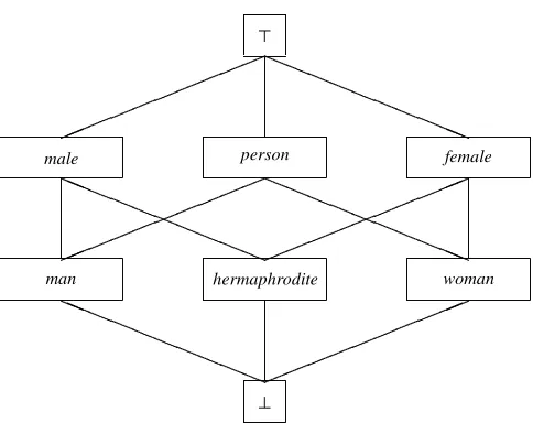
Sorts also come with a GLB operation^. For example,
person^male=man;
male^female=hermaphrodite;
man^woman=?;
etc., which can be visualized as shown in Figure 1. We will refer back to this figure in several examples to come.
Features (or attribute labels) are also symbols and used to build -terms by attaching attributes to sorts. The set of feature symbols is calledF. We will use words and natural numbers as features. The latter are handy to specify attributes by positions as subterms in first-order terms. Examples of feature symbols are age, spouse,1,2.
-Terms
Basic -terms are the simplest form of -terms. They are:
variables; e.g., X;Y;Z; . . .
sorts; e.g., person;int;true;3:5;>; . . . tagged sorts; e.g., X :>; Y : person; . . .
Stand-alone variables are always implicitly sorted by >, and stand-alone sorts are always implicitly tagged by some variable occurring nowhere else. Thus, one might say that a basic
?
man hermaphrodite woman
male person female
[image:14.612.92.334.70.262.2]> a a a a a a a a a a ! ! ! ! ! ! ! ! ! ! a a a a a a a a a a ! ! ! ! ! ! ! ! ! ! ! ! ! ! ! ! ! ! ! ! a a a a a a a a a a ! ! ! ! ! ! ! ! ! ! a a a a a a a a a a
Figure 1. A partial order of sorts
-term is always of the form variable : sort.
Features are used to build up more complex -terms. Thus, the following -term is obtained from the -term person by attaching the feature age typed by the -term int:3
X : person(age)I : int):
The sort at the root of a -term, here person, is called its principal sort. A -term can be seen as a record structure. Features correspond to field identifiers, and fields are, in turn, associated to -terms. These are flexible records in the sense that variably many fields may be attached to the principal sort. For example, we can augment the -term above with another feature:
X : person(age)I : int;
spouse)Y : person(age)J : int)):
This -term denotes the set of all objects X of sort person (in the intended domain), whose value I under the function age is of sort int, whose value Y under the function spouse is of sort person, and the value J of Y under the function age is of sort int.
The following -term is more specific, in the sense that the above set becomes smaller if one further requires that the values I and J coincide; namely, age(X)=age(spouse(X)):
X : person(age)I : int;
spouse)Y : person(age)I)):
3To illustrate the -term ordering, we will give a decreasing matching sequence of -terms going from more
It denotes the subset of individuals in the previous set of person’s whose age is the same as their spouse’s. This -term uses a coreference thanks to sharing the variable I. The next -term is even more specific, since it contains an additional (circular) coreference; namely, X=spouse(spouse(X)):
X : person(age)I : int;
spouse)Y : person(age)I; spouse)X)):
It denotes the set of all individuals in the previous set whose spouse’s spouse is the individual in question. Note that only variables that are used as coreference tags need to be put explicitly; i.e., those that occur at least twice.
To be well-formed, the syntax of a -term requires three conditions to be satisfied: (1) the sort ? may not occur; (2) at most one occurrence of each variable has a sort; (3) all the features attached to a sort are pairwise different. These conditions are necessary to ensure that a -term expresses coherent information. For example, X : man(friend) X : woman), violating Condition (2), is not a -term, but X : man(friend)X)is.
As for ordering, a -term is made more specific through:
sort refinement; e.g., X : intU :>;
adding features typed by -terms; e.g., X :>(age)int)U :>; adding coreference; e.g., X :>(likes)X)U :>(likes)V).
Note that, as record structures, -terms are both record types and record instances. In addition, they allow mixing type and value information. Finally, they also permit constraining records with equations on their parts.
-Terms as graphs
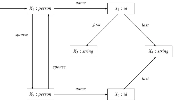
There is a straightforward representation of a -term as a rooted directed graph. Let us assume that every variable is explicitly sorted (if necessary, by the sort>) and every sort is explicitly tagged (if necessary, by a single-occurrence variable). The nodes of the graph are the variables, their labels are the corresponding sorts; for every feature mapping one variable X to another one Y there is an arc(X;Y)labeled by that feature. One node is marked as the root (whose label is called the root sort or the principal sort of the -term).
For example, the -term:
X1: person(name)X2: id(first)X3: string; last)X4: string);
spouse)X5: person(name)X6 : id(last)X4); spouse)X1)).
- X
1: person
X5: person
X3: string X4: string
X2: id
X6: id
name
-name
-spouse
?
spouse
6
first last
@ @
@ @
@ @ R
last
[image:16.612.92.393.90.269.2]
Figure 2. An OSF-Graph
-Terms as values
One particular interpretation is readily available for -terms. Namely, the syntactic interpre-tation whose domain is the set of all -terms. Note that -terms have a dual personality. They are syntactic objects (graphs) representing the values of the domain of , and they also are types which denote sets. In the particular case of the interpretation , they denote subsets of the domain of ; i.e., sets of -terms. We shall see this dual view does not lead to paradox, au contraire.
In the interpretation , a sort s2Sdenotes the set of all -terms whose root sort is a subsort of s. A feature`2Fdenotes the function mapping a -term to its sub- -term under that feature, or to>, if there is none.
Thus, a sort denotes the set of all -term values which, as -term types, are more specific than the basic -term s. In fact, it is possible to show that in general a -term denotes the set of all -terms which are more specific than the -term itself. This is the “ -terms as filters” principle established in [5]. It yields directly the fact that the partial orderingon -terms is exactly set-inclusion of the sets denoted by the -terms in the -term domain.
Feature trees as values
We obtain two other examples of OSF-algebras when we “compress” the -term domain by identifying values. In a first step, we say that two -terms which are equal up to variable renaming represent the same value of the domain, or: two isomorphic graphs are identified. We call the OSF-algebra hereby obtained0.
unfolding. Hence, unfolding an OSF-graph yields what we call a feature tree. Such a tree is one whose nodes are labeled with sorts and whose edges are labeled with features. Therefore, we can also identify -terms which represent the same rational tree. The domain hereby obtained is essentially the feature tree structureT introduced first in [7] and [8].
Unification of -terms
We say that 1is unifiable with 2if 1^ 26=?; i.e., if there exist -terms with non-empty denotations which are more specific than both 1 and 2. Then, one can show that there exists a unique (up to variable renaming) -term which is the most general of all these, the ‘greatest lower bound’ (GLB) of 1and 2, written = 1^ 2.
For the set denotation of -terms,^is exactly set intersection. An important result illustrating the significance of the -term interpretation is that 1is unifiable with 2 if and only if the intersection of the two sets denoted by 1and 2in the -term domain is non-empty.
Constraints and -terms
We also view a -term logically as a constraint formula by flattening it into what we call its dissolved form. For ease of notation, we shall write(X : ) to indicate that the root variable of the -term is X.
More precisely, the -term X : s(`1)(X1 : 1);. . .;`n)(Xn : n)) corresponds to the conjunction of the constraint X : s & X:`1
:
= X1 & X:`n :
= Xn and of the constraints corresponding to 1;. . .; n. A basic -term X : s corresponds to the sort constraint X : s. For example, the -term:
X : person(likes)X; age)Y : int)
is identified with the constraint:
X : person & X:age :
=Y & Y : int & X:likes : =X:
Thus, the constraint is a conjunction of atomic sort constraints of the form X : s and atomic feature constraints of the form X:`
:
=Y. The interpretation of the sort and feature constraints over the intended domain is straightforward, given that sorts are interpreted as subsets of the domain and features as unary functions over the domain.
A value lies in the set denoted by the -term in an interpretation I if and only if the constraint X :
Rules for unification
Unifying (X1 : 1) and (X2 : 2) amounts to deciding satisfiability of the conjunction
1 & 2 & X1 :
=X2. Thus, the unification algorithm can be specified in terms of constraint normalization rules. A constraint containing the conjunction over the line is rewritten into an equivalent constraint by replacing this conjunction by the constraint under the line. We only need four rules that are illustrated schematically on an example below. (Refer to the sorts of Figure 1.)
Equality:
. . . X : person & U : male & U : =X . . . . . . X : person & X : male & U :
=X . . .
Sorts:
. . . X : person & X : male . . . . . . X : man . . .
Features:
. . . X:likes :
=Y & X:likes : =V . . . . . . X:likes
:
=Y & V : =Y . . .
Clash:
. . . X :? . . .
?
One can show that a constraint is satisfiable if and only if it is normalized to a constraint different from the false constraint?. If we identify every constraint containing a sort constraint of the form X :?with the false constraint, we omit the clash rule.
In particular, the -terms(X1: 1)and(X2: 2)are unifiable if and only if 1 & 2& X1 : =X2 is normalized into a constraint different from?. This constraint corresponds, apart from its equalities (between variables), to the -term (unique up to variable renaming) 1^ 2.
2.2 Relative simplification
We use the framework of first-order logic to transform the combined entailment/disentailment problem into one that can be solved by the relative simplification algorithm.
Matching and entailment
In the Concurrent Constraint Logic Programming framework, the matching problem generalizes to the entailment problem; namely, whether the actual constraint, also called context, entails the formal constraint, also called guard [20, 23].
First observe that, for example, the first-order term t1 = f(Z;f(Y;Y)) matches the term t2=f(W;V), and that the implication:
8X8Y8Z X :
=f(Z;f(Y;Y))!9U9V9W(X :
=U & U :
=f(W;V))
is valid. Generally, the term t1 matches t2 (noted t1 t2) if and only the implication X :
=t1 ! 9U9V (X :
= U & U :
=t2) is valid, where V stands for all variables of t2. More shortly, X :
=t1entails X :
=U & U : =t2.
Note, however, that there is an essential difference between -term matching and first-order term matching. For example, the term f(a;a)matches the term f(V;V). This is true because first order terms denote individuals. This is no longer true in LIFE. For example, the -term X : f(1)Y : int;2)Z : int)does not match the -term U : f(1)V;2)V). Indeed, the presence of two occurrences of the same sort does not entail that the individuals in that sort be equal. Therefore, X : s(1) 1;2) 2)is less specific than the -term U : s(1)V;2)V) only if the root variables of 1and 2are identical (or bound together).
This does not mean that values and operations on them are not available in LIFE.4 What the above point illustrates is that to recognize that a sort is a fully determined value, and hence to enforce identity of all its distinct occurrences, one needs this information declared explicitly, in effect adding an axiom to the formalization of such sorts. So-declared extensional sorts can then be treated accordingly thanks to an additional inference rule (being a minimal non-bottom sort is not sufficient). Without this rule, however, equality of distinct occurrences cannot be entailed and the behavior illustrated is the only correct one. The point of this paper being independent if this issue, we shall omit this additional rule.
The fact that(X : 1) (U : 2), i.e., the -term(X : 1) matches the -term(U : 2), translates into the fact that the corresponding constraint 1entails the constraint 2& U :
=X. This means that the implication 1!9U;V;W . . . 2 & U
:
=X is valid. Here,9U;V;W . . . indicates that all local variables are existentially quantified. The global variables are universally quantified.
Entailment of general constraints
We will now give a precise explanation of a fact which is well-known for constructor terms. An actual parameter t1matches a formal parameter t2 if and only if the unification of the two terms binds only variables of t2, but no variable of t1. In other words, only local, but no global, variables are instantiated.
4Of course, one can use actual values of sort int, real, or string in expressions with their usual operations as
The unification of the term t1 =f(Z;f(Y;Y))and the term t2 = f(W;V)yields the variable bindings W :
=Z and V :
=f(Y;Y). On the other hand, the conjunction:
X :
=f(Z;f(Y;Y))& U :
=X & U :
=f(W;V)
is equivalent to:
X :
=f(Z;f(Y;Y))& U : =X & V
:
=f(Y;Y)& W : =Z
;
and the last part of this conjunction is valid if the local variables U;V;W are existentially quantified.
This is the general principle which underlies the relative simplification algorithm. Namely, the actual constraint 1entails 2 & U :
=X if and only if the following holds. Their conjunction
1& 2& U :
=X is equivalent to the conjunction 1& 0
2of the actual constraint 1and a
constraint 0
2which is valid if existentially quantified over the local variables. In our case, 0
2
will be a conjunction of equalities binding local to global variables. Formally,
j= 1!9U;V;W;. . . 2& U : =X
if and only if there exists a formula 0
2such that:
j=( 1& 2 & U :
=X)$( 1& 0
2) and j=9U;V;W . . . 0
2:
This statement is correct since validity of the implication 1!9U 2& U :
=X is the same as the validity of the equivalence 1&(9U 2& U
: =X)
$ 1. This fact is analogous to the fact that a set is the subset of another one if and only if it is equal to the intersection of the two. The conditionj=9U;V;W . . .
0
2 in the statement expresses that 1 &(9U;V;W;. . . 0
2)is equivalent to 1.
Towards relative simplification
Operationally, in order to show that(X : 1) (U : 2) holds, it is sufficient to show that the conjunction 1 & 2 & U :
= X is equivalent to 1 & 0
2, where 0
2 is some constraint
which, existentially quantified over the variables of 2, is valid. In our case, again, 0
2will be
a conjunction of equalities binding variables of 2to variables of 1.
Therefore, in order to test (X : 1) (U : 2), we will apply successively the unification rules on the constraint 1& 2 & U :
=X if they do not modify 1. We obtain three kinds of transformations which are illustrated schematically below. (Refer to the sorts of Figure 1.)
Equality:
. . . X :
=Y & U : =X . . . . . . X :
Sorts:
. . . X : man & U :
=X & U : person . . . . . . X : man & U :
=X . . .
Features:
. . . X:likes :
=Y & U :
=X & U:likes : =V . . . . . . X:likes
:
=Y & U :
=X & V : =Y . . .
The equality rule is derived from the corresponding unification rule, which has to be restricted to modify only the formal constraint. If the actual constraint contains an equality between two global variables, then one of them may be eliminated for the other. A global variable is never eliminated for a local one.
The sort rule corresponds to two applications of unification rules, first the elimination of the local by the global variable, and then the reduction of two sort constraints on the same variable (here X : man & X : person) to one sort constraint (namely X : man^person). Clearly, if the “global sort” is a subsort of the “local sort” then this application does not modify the global constraint. The feature rule works quite similarly.
For example, the rules above can be used to show that the -term:
1 X : man(likes)Y : person;age)I : int)
matches the -term:
2 U : person(likes)V):
Namely, the constraint 1& 2& U : =X :
X : man & X:likes :
=Y & Y : person & X:age :
=I & I : int & U : person & U:likes
: =V & U :
=X
is normalized into:
X : man & X:likes :
=Y & Y : person & X:age :
=I & I : int & V :
=Y & U : =X;
that is,
1 & V :
=Y & U : =X:
Clearly,9U9V V :
=Y & U : =X
is valid. Therefore, the constraint 1 entails the constraint
Relative simplification for entailment
The rules above are such that 1 & rewrites to 1 & 0
; i.e., the global constraint 1 is not modified by the simplification. In this case, we say that the constraint simplifies to 0 relatively to the actual constraint 1. In other words, 1acts as a context relatively to which simplification of is carried out. In general, this context formula may be any formula. Hence, we can reformulate the rules above as relative-simplification rules. We use the notation 0 [
] to mean that is simplified into 0
relatively to the context formula. Schematically,
Equality:
. . . U : =X . . . . . . U :
=Y . . .
[ . . . X : =Y . . . ]
Sorts:
. . . U :
=X & U : person . . . . . . U :
=X & . . .
[ . . . X : man . . . ]
Features:
. . . U :
=X & U:likes : =V . . . . . . U :
=X & V : =Y . . .
[ . . . X:likes : =Y . . . ]
Using these rules, the constraint 2 U :
=X & U : person & U:likes :
=V in the previous example simplifies to 0
2 U
: =X & V
:
=Y relatively to:
1X : man & X:likes :
=Y & Y : person & X:age :
=I & I : int:
Invariance of relative simplification is the following property. If simplifies to 0
relatively to, then the conjunction of withis equivalent to the conjunction of
0
with.
This invariance justifies the correctness of the relative simplification algorithm with respect to entailment. Namely, if simplifies to 0
relatively to, and if 0
consists only of equations binding local variables, thenentails .
Proof of completeness of the algorithm needs the assumption that the setF of features is infinite. Note that exactly thanks to the infiniteness ofF our framework accounts for flexible records; i.e., the indefinite capacity of adding fields to records.
Relative simplification for disentailment
match the formal one even when further instantiated; e.g., when further constraints are attached as conjuncts. Logically, this amounts to saying that a context formuladisentails a guard constraint if and only if the conjunction & is unsatisfiable. In terms of relative simplification,disentails if and only if simplifies to the false constraint?relatively to.
For example, X : male is non-unifiable with U : woman.5 The constraint U : woman & U : =X simplifies to?relatively to the constraint X : male, since woman^male=?, using a rule of the form indicated below, and then the Clash rule.
Sorts:
. . . U :
=X & U : woman . . . . . . U :
=X & U : woman^male . . .
[ . . . X : male . . . ]
The following example shows that a sort clash cannot always be detected by comparing sorts in the formal constraint one by one with sorts in the actual constraint; i.e., one needs several steps with intermediate sort intersections.
The -term Z : >(likes)X : male;friend)Y : female) is non-unifiable with the -term W : >(likes)U : person;friend)U). The constraint X : male & Y : female disentails the constraint U
:
=X & U :
=Y & U : person. Operationally, the constraint simplifies to?relatively to the context. Here are the steps needed to determine this:
. . . U :
=X & U :
=Y & U : person . . .
. . . U :
=X & U :
=Y & U : person^male . . .
. . . U :
=X & U :
=Y & U : man^female . . .
?
There is an issue regarding the enforcing of functionality of features in the simplification of a constraint relatively to a context. This may be explained as follows. Let us suppose that two global variables X and Y become bound to the same local variable U. Then,
the contextentails the constraint only ifcontains X :
=Y; and,
the contextdisentails the constraint if the same path of features starting from X and Y, respectively, leads to variables X0
and Y0
, respectively, whose sorts are incompatible.
There are essentially two cases, depending on whether a new local variable has to be introduced or not. Each case is illustrated in the next two examples.
The -term:6
Z :>(likes)X :>(age)I1 : poseven); friend)Y :>(age)I2: posodd))
5Refer to the sorts of Figure 1. 6We assume that poseven
is non-unifiable with the -term:
W :>(likes)U; friend)U)
That is, the constraint disentails the constraint . Operationally, with the context, the constraint simplifies, in a first step, to:
W :
=Z & U :
=X & U : =Y:
Then, using the rule:
. . . U :
=X & U : =Y . . . . . . U :
=X & U : =Y & J
: =I1& J
: =I2 . . .
[ . . . X:age :
=I1& Y:age : =I2 . . . ]
where J is a new variable, to:
W :
=Z & U :
=X & U : =Y & J
: =I1& J
: =I2
and finally to?, since the sorts of I1and I2 (poseven and posodd) are incompatible.
The rules enforce the following property: a global variable is never bound to more than one local variable. Therefore, if the variable X or the variable Y is already bound to a local variable, no new local variable must be introduced. This is illustrated by the second example.
The -term:
Z :>(likes)X :>(age)I1 : poseven); friend)Y :>(age)I2 : posodd); age)I1)
is non-unifiable with the -term:
W :>(likes)U;
friend)U(age)J); age)J):
Operationally, with the context, the constraint simplifies, in a first step, to:
W :
=Z & U :
=X & U : =Y & J
: =I1:
. . . U :
=X & U : =Y & J
: =I1 . . . . . . U :
=X & U : =Y & J
: =I1 & J
: =I2 . . .
[ . . . X:age :
=I1& Y:age : =I2 . . . ]
where J is a new variable, to:
W :
=Z & U :
=X & U : =Y & J
: =I1& J
: =I2
and finally to?, for the same reason as above.
In order to be complete with respect to disentailment, the algorithm must keep track of all pairs of variables(X;Y);. . .;(X
0 ;Y
0
)whose equality is induced by the binding of X and Y to the same local variable. That is, it must propagate equalities along features. In our presentation, it will be conceptually sufficient to refer explicitly to the actual equalities binding the global variables to a common local variable. Practically, this can of course be done more efficiently.
Specifying the relative simplification algorithm
If & U :
=X simplifies to 0
relatively toand no relative-simplification rule can be applied further, then:
entails & U :
=X; formally,
j=!9U;V;W . . .( & U : =X);
if and only if 0
, with the variables of existentially quantified, is valid; formally:
j=9U;V;W . . . 0
:
disentails & U :
=X; formally:
j=!:9U;V;W . . .( & U : =X);
if and only if 0 =?.
This test is incremental. Namely, every relative simplification of the constraint to some constraint 0
relatively to the context is also a relative simplification relatively to an incremented context&
0
, for any constraint 0
.
Recapitulating, our original goal was a simultaneous test of matching and non-unifiability for two given -terms 1 and 2. This test was recast as a test of entailment and disentailment for the constraints to which the -terms dissolve. Namely, if X and U are the root variables of
1and 2, respectively, the test whether 1entails or disentails 2& U : =X.
In our setting, the entailment test succeeds if and only if 0
2 is a conjunction of matching
equations; i.e., of the form 0
2 U
:
=X & V :
=Y & W :
3 Background
We introduce briefly the notions that we have used informally in Section 2. For a thorough investigation of these notions, the reader is referred to [6, 5].
We start with the notion of OSF-algebras. They are the semantic structures interpreting complex data objects built out of features and partially-ordered sorts. Mathematically, an OSF-algebra formalizes access into the parts making up a piece of datum as well as their categorization. We then introduce OSF-constraints. They are important since, although they are formal objects which are part of a logical formalism, they are also quite primitive to constitute a low-level implementation logic.7 We then formalize -terms as they not only constitute a syntactically pleasant and convenient surface language for data objects in LIFE, but also comprise a syntactic OSF-algebra. Namely, they are representations of values of the domain of the standard interpretation. Finally, we summarize a few facts about this formalism that are relevant as related to the global contents of the paper.
3.1 OSF-algebras and OSF-constraints
The building blocks of OSF-algebras are sorts and features.
An order-sorted feature signature (or simply OSF-signature) is a tuplehS;;^;Fisuch that:
Sis a set of sorts containing the sorts>and?;
is a decidable partial order onSsuch that?is the least and>is the greatest element; hS;;^iis a lower semi-lattice (s^s
0
is called the greatest common subsort of sorts s and s0
);
F is a set of feature symbols.
An OSF-signature has the following interpretation. An OSF-algebra over the signature
hS;;^;Fiis a structure:
A=hD A
; s A
s2S ; `
A
`2F i
such that:
D
A
is a non-empty set, called the domain ofA(or, universe);
for each sort symbol s inS, s A
is a subset of the domain; in particular, > A
=D
A and
? A
=;;
the greatest lower bound (GLB) operation on the sorts is interpreted as the intersection; i.e.,(s^s
0 )
A =s
A \s
0A
for two sorts s and s0 inS.
for each feature`inF,` A
is a total unary function from the domain into the domain; i.e.,`
A : DA
7!D A
;
7In fact, the reader familiar with implementation techniques of Prolog [2] should recognize that they are of the
The notion of OSF-algebra calls naturally for a corresponding notion of homomorphism preserving structure appropriately. Namely,
Definition 1 (OSF-Homomorphism) An OSF-algebra homomorphism :A7!Bbetween two OSF-algebrasAandBis a function: D
A 7!D
B
such that:
`
A (d)
=`
B (d)
for all d2D A
;
s
A
s B
.
It is straightforward to verify that OSF-algebras together with OSF-homomorphisms form a category. We call this category OSF.
LetVbe a countably infinite set of variables.
Definition 2 (OSF-Constraint) An atomic OSF-constraint is one of:
X : s,
X
: =X
0 ,
X:` : =X
0 ,
where X and X0
are variables inV, s is a sort inS, and`is a feature inF. An OSF-constraint is a conjunction of atomic OSF-constraints.
One reads the three forms of atomic OSF-constraints as, respectively, “X lies in sort s,” “X is equal to X0
,” and “X0
is the feature `of X.” The set Var()of variables occurring in an OSF-constraintis defined in the standard way. OSF-constraints will always be considered equal if they are equal modulo the commutativity, associativity and idempotence of conjunction “&.” Therefore, a constraint can also be formalized as the set consisting of its conjuncts. As usual, the empty conjunction corresponds to the propositional constant interpreted as true.
LetAbe an OSF-algebra. We call Val(A)=f:V 7!D A
gthe set of all possible valuations in the interpretationA. The semantics of OSF-constraints is straightforward.
GivenA is OSF-algebra, an OSF-constraintis satisfiable in A, if there exists a valuation
:V 7!D A
such thatA;j=, where:
A;j=X : s if and only if (X)2s A
;
A;j=X :
=Y if and only if (X)=(Y); A;j=X:`
:
=Y if and only if ` A
((X))=(Y); A;j=&
0
if and only if A;j=andA;j= 0
:
3.2 -Terms
Definition 3 ( -Term) A -term is an expression of the form:
X : s(`1) 1;. . .;`n) n)
where
X is a variable inVcalled the root of ;
s is a sort different from?inS;
`1;. . .;`nare pairwise different features inF, n0; 1;. . .; nare again -terms; and,
no variable Y occurring in is the root variable of more than one non-trivial -term (i.e., different than Y :>).
Note that the equation above includes n=0as a base case. That is, the simplest -terms are of the form X : s.
We can associate to a -term =X : s(`1) 1;. . .;`n) n)the OSF-constraint:
( )=X : s & X:`1 :
=Y1 & . . . & X:`n :
=Yn &( 1)& . . . &( n)
where Y1;. . .;Yn are the roots of 1;. . .; n, respectively. We say that the OSF-constraint
( )is obtained from dissolving the -term , and refer to the OSF-constraint as the dissolved -term. We will often deliberately confuse a -term with its dissolved form ( ) and simply refer to( )simply as .
Given the interpretationA, the denotation [[ ]] A;
under a valuation :V7! D A
of a -term with root X is given as:
[[ ]]A;
=fd2D A
j(X)=d; A;j= g:
Note that this is either the singletonf(X)gor the empty set.
The type-as-set denotation of a -term is defined as the set of domain elements:
[[ ]]A =
[
2Val(A) [[ ]]A;
:
This amounts to saying that:
[[ ]]A
=fd2D A
jthere exists2Val(A)such that(Z)=d; andA;j=9X Z : g
where Z is a new variable not occurring in ,X =Var( ), Z : stands for Z :
A -term with root X corresponds to a unique rooted graph g which is the direct translation of the constraint together with an indication of the root. The nodes of g are exactly the variables of . A node Z is labeled by the sort s if the conjunction contains a non-trivial sort constraint Z : s, and by the sort>, otherwise. For every feature constraint Y:`
: =Z the graph g has a directed edge(Y;Z)which is labeled by the feature`. The root of g is the node X. Clearly, g is the natural graphical representation of .8
3.3 Syntactic interpretations
Among all OSF-algebras, there are those whose domain elements are concrete data structures. We call these syntactic interpretations. We will now present three important examples obtained directly from the syntactic expressions of -terms. They turn out to be canonical interpretations for OSF-constraints.9
The most immediate syntactic OSF-interpretation is the OSF-algebra of -terms. The domain of is the set of all -terms, up to graph representation. That is, we identify -terms as values of if they are represented by the same graph. For example, the two -terms Y : s(`1)X : s
0
;`2)X) and Y : s(`1)X;`2)X : s 0
) clearly correspond to the same object. Indeed, they have the same OSF-graph representation.
Sorts s2Sare interpreted as:
s =f 2Djs 0
s; where s 0
is the root sort of the graph of g;
and features ` 2F are interpreted as functions` : D 7! D as follows. Let be a -term and g its graph. If(X;Y) is the edge of g labeled by`, then `(g)is the -term represented by the maximally connected subgraph g0
of g rooted at the node Y. That is, g0
is obtained by removing all nodes and edges which are not reachable by a directed path from the node Y.
If X does not have the feature`, i.e., there is no outgoing edge from the root of g labeled `, then`is the -term Z
`; :
>, for a new variable Z
`; uniquely determined by the feature `and the -term .
For example, taking =X :>(`1)Y : s;`2)X), we have`
1( )=Y : s,`
2( )= , and
`
3( )=Z `3; :
>.
We obtain two other examples of OSF-algebras when we factorize the -term domain by further identifying values. The first one identifies two -terms which are equal up to variable renaming. The obtained domain obviously spans an OSF-algebra. We call this OSF-algebra0.
The second one is obtained from0by further identifying two -terms if their (possibly infinite) tree unfoldings are equal. A tree unfolding is obtained from a -term by associating a unique node to every feature path. It is well known that a rooted directed graph represents a unique rational tree [14]. In our case, we obtain trees whose nodes are labeled by sorts and whose
8Refer to Figure 2 on Page 8 for an example.
edges are labeled by features. We call these (rational) OSF-trees. It is again clear that the set of all OSF-trees spans an OSF-algebraT.
10
Formally, OSF-algebras can also be introduced as logical structures, namely models providing interpretations for the sort symbols as unary predicates and the feature symbols as unary functions, which satisfy the Sort Axiom saying, for all sorts s and s0
,
X : s & X : s0
! X : s^s 0
:
Furthermore, both0andT satisfy a Constructibility Axiom stating essentially the satisfiability of any OSF-constraintcoming from dissolving a -term . More precisely, ifX =Var() and, for i=1;. . .;n, Xi:`i
:
=Y 62for any variable Y, and Yi62Var(), and Xi 2X, then this axiom states the validity of:
8Y1:. . .8Yn:9X:& X1:`1 :
=Y1 & . . . & Xn:`n : =Yn:
The constructibility axiom is a generalization of the axiom of functionality which is valid for first-order terms. Namely, the axiom which guarantees that, given a constructor symbol f of rank n, an individual X =f(Y1;. . .;Yn)exists if individuals Yi exist, i=1;. . .;n. Formally, taking=X : f ,
8Y1:. . .8Yn:9X:X : f & X:1 :
=Y1 & . . . & X:n : =Yn:
The form we give for constructibility is indeed more general than plain functionality since it states the existence of something which is not valid for first-order terms; e.g., self-referential individuals. For example, 9X:X:`
:
=X is obtained as an instance of our axiom by taking n=0and=X:`
: =X.
3.4 OSF-unification
We describe next how to determine whether an OSF-constraint is consistent; i.e., if it is satisfiable in some OSF-algebra A—and, therefore, in particular in . Unification of two
-terms reduces to this problem.
Definition 4 (Solved OSF-Constraints) An OSF-constraint is called solved if for every variable X,contains:
at most one sort constraint of the form X : s, with?<s;
at most one feature constraint of the form X:` :
=Y for each`; and,
no other occurrence of the variable X if it contains the equality constraint X : =Y.
10
T is essentially the feature tree structure of [7] and [8, 25]. The difference lies in our using partially-ordered
In [6, 5], we show that an OSF-constraint in solved form is always satisfiable. Now, by Definition 3, the OSF-constraint obtained as the dissolved form of any -term is de facto in solved form.11 Hence, such a constraint is always satisfiable. It is so, in particular, in the canonical interpretation with, interestingly enough, the valuation that assigns to each variable X in the value in D that is the very -term rooted in X in . For this reason, a -term can also be seen as a variable substitution.
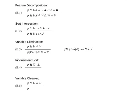
Given an OSF-constraint , it can be normalized by choosing non-deterministically and applying any applicable rule among the transformations rules shown in Figure 3 until none
Feature Decomposition:
(B.1)
& U:` :
=V & U:` : =W & U:`
: =V & W
: =V
Sort Intersection:
(B.2)
& U : s & U : s0
& U : s^s 0
Variable Elimination:
(B.3)
& U : =V [V=U] & U
: =V
if U2Var( )and U6=V
Inconsistent Sort:
(B.4)
& X :?
?
Variable Clean-up:
(B.5)
[image:31.612.83.513.203.522.2]& U : =U
Figure 3. Basic simplification
applies. A rule transforms the numerator into the denominator. The expression[X=Y] stands for the formula obtained fromafter replacing all occurrences of Y by X.
Theorem 1 (OSF-Constraint Normalization) The rules of Figure 3 are solution-preserving, finite terminating, and confluent (modulo variable renaming). Furthermore, they always result in a normal form that is either the false constraint?or an OSF-constraint in solved form.
11More precisely, this is true if we forget superfluous trivial sort constraints of the form X :
For our purposes, the constraintto be normalized will be of the form 1 & 2& X1 : =X2; i.e., the conjunction of the dissolved -terms 1and 2together with an equation identifying their root variables X1 and X2. Ifnormalizes to the false constraint, then the two -terms are non-unifiable. Otherwise, the resulting solved OSF-constraint is a conjunction of equality constraints and of the dissolved form of some -term. This -term is the most general unifier of 1 and 2, up to variable renaming. We shall see that this -term has two equivalent order-theoretic characterizations (cf., Propositions 3 and 4).
3.5 OSF-orderings and semantic transparency
In this section, we first introduce the notion of endomorphic approximation which captures precisely and elegantly object inheritance. We also show how it relates to the logic and type views.
Endomorphisms on a given OSF-algebra A, i.e., homomorphisms from A to A, induce a natural partial ordering.
Definition 5 (Endomorphic Approximation) On each OSF-algebra A an approximation preorderv
Ais defined such that, for two elements d and e in D A
, d approximates e if and only if e is an endomorphic image of d. Formally,
dv Ae iff
(d)=e for some endomorphism :A7!A:
We shall omit subscriptingv
Aand write
vwhenA=. Notice that this ordering on -terms as values of the domain of translates into an information-theoretic approximation ordering on
-terms as types.
We note that endomorphisms on are graph homomorphisms with the additional sort-compatibility property. A node labeled with sort s is always mapped into a node labeled with s or a subsort of s. An edge labeled with a feature is mapped into an edge labeled with the same feature. Thus, endomorphic approximation captures exactly object-oriented class inheritance. Indeed, if an attribute is present in a class, then it is also present in a subclass with a sort that is the same or refined. Since features are total functions, this also takes care of introducing a new attribute in a subclass: it refines >. Note also, that the restriction of to the set of nodes defines a variable binding; it corresponds to the notion of a matching substitution for first-order terms.
The following fact was established in [6, 5].
Proposition 1 ( -Terms as Filters) The denotation of a -term in is the set of all -terms it approximates; i.e.,
[[ ]] =f 0
2Dj v
The next ordering is the type ordering on -terms which we informally called “more specific than” in Section 1.2 and Section 2.
Definition 6 ( -Term Subsumption) A -term is subsumed by a -term 0
if and only if the denotation of is contained in that of 0
in all interpretations. Formally,
0
iff [[ ]]A [[
0 ]]A
for all OSF-algebrasA.
In fact, it is sufficient to limit the above statement to the OSF-algebra only; i.e., [[ ]][[ 0
]].
The next and last ordering is a logical ordering on -terms. We state it here in less general terms than in [6, 5].
Definition 7 ( -term Entailment) A -term entails a -term 0
if and only if, as constraints, implies the conjunction of 0
and X : =X
0
; more precisely,
0
iff j= !9U (X : =X
0 & 0
)
where X, X0
are the roots of and 0
andU =Var( 0
).
It is again sufficient to state the validity of the implication in the OSF-algebra only (namely, using j=). This is not true in the more general wording and holds here only because the constraints are obtained by dissolving -terms and their root variables are bound together.
Proposition 2 (Semantic Transparency of Orderings) The following are equivalent:
v
0
is an approximation of 0 ;
0
0
is a subtype of ;
0
entails
0 ;
[[ ]] [[ 0
]] the set of -terms filtered by is contained in that filtered by 0 .
The following two propositions are straightforward. Let 1 and 2 be two -terms with variables renamed apart; i.e., such that Var( 1)\Var( 2)=;. Let X1and X2be their respective root variables. Letbe the normal form of the OSF-constraint 1& 2& X1
: =X2.
Proposition 3 ( -Term Unification) The normal formis the false constraint if and only if [[ 1]]A
\[[ 2]] A
= ;, for all OSF-algebrasA. Otherwise, is the conjunction of equality constraints and of the dissolved version of some -term . This -term is the-GLB of 1 and 2up to variable renaming; i.e., [[ ]]A
=[[ 1]] A
\[[ 2]] A
.
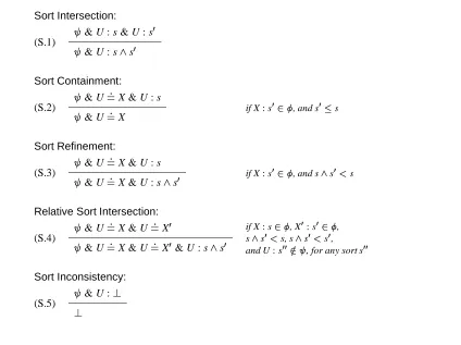
4 Entailment and disentailment of OSF-constraints
This section deals formally with all the apparatus presented and used informally in Section 2.2.
In the following, we useas the context formula. It is assumed to be an OSF-constraint in solved form, although not necessarily coming from dissolving a single -term. The variables inare global. We shall useX to designate the set of global variables Var()and the letters X, Y, Z, . . . , for variables inX. We use , a dissolved -term, as the guard formula. The variables in are local to ; i.e., Var()\Var( )=;. We shall useU to designate the set of local variables Var( )and the letters U, V, W, . . . , for variables inU. The letter U will always designate the root variable of . We also refer toas the actual parameter, and to as the formal parameter. By extension, we will often use the qualifiers global/local, actual/formal, and context/guard, with all syntactic entities; e.g., variables, formulae, constraints, or sorts.
We investigate a proof system which decides two problems simultaneously:
the validity of the implication8X !9U:( & U : =X)
;
the unsatisfiability of the conjunction& & U : =X.
The first test is called a test for entailment of the guard by the context, and the second, a test for disentailment. This second test is equivalent to testing the validity of the implication
8X !:9U:( & U : =X)
.
Since both tests amount to deciding whether the context implies the guard or its negation, all local variables are existentially quantified and all global variables are universally quantified.
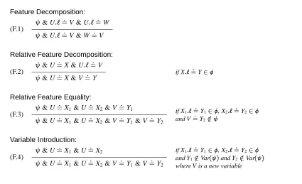
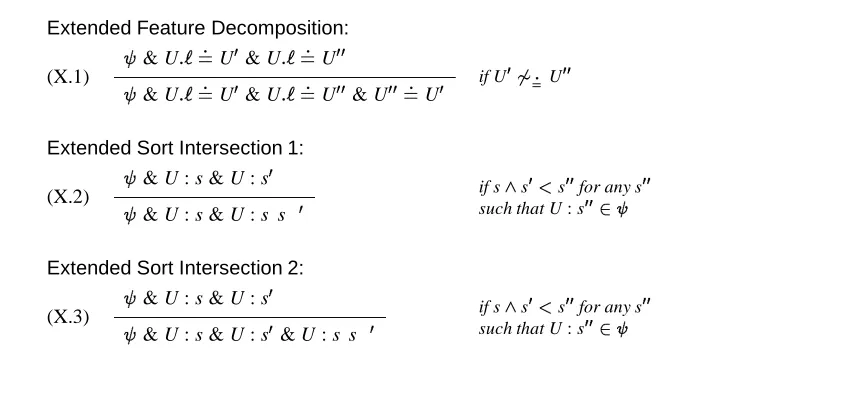
The relative-simplification system for OSF-constraints is given by the rules in Figures 4, 5, and 6. An OSF-constraint simplifies to 0
relatively toby a simplification ruleif 0 is an instance ofand the applicability condition (on and on ) is satisfied. We say that simplifies to 0
relatively toif it does so in a finite number of steps.
The relative-simplification system preserves an important invariant property: a global variable never appears on the left of a variable equality constraint in the formula being simplified. Thus, an equality U :
= X is a directed relation binding the local variable U to the global variable X. Furthermore, a global variable is never eliminated by a local one, or vice versa.
A set of bindings Ui
:
= Xi, i = 1;. . .;n is a functional binding if all the variables Ui are mutually distinct.
The effectuality of the relative-simplification system is summed up in the following statement:
Effectuality of relative-simplification The solved OSF-constraint entails (resp., disentails) the OSF-constraint9U:(U
:
=X & )if and only if the normal form 0
of & U :
=X relatively tois a conjunction of equations making up a functional binding (resp., is the false constraint 0
Feature Decomposition:
(F.1)
& U:` :
=V & U:` : =W
& U:` : =V & W
: =V
Relative Feature Decomposition:
(F.2)
& U :
=X & U:` : =V
& U : =X & V
: =Y
if X:` : =Y2
Relative Feature Equality:
(F.3)
& U :
=X1& U :
=X2& V : =Y1 & U :
=X1& U :
=X2& V :
=Y1& V : =Y2
if X1:` :
=Y12, X2:` : =Y22
and V :
=Y22=
Variable Introduction:
(F.4)
& U :
=X1& U : =X2 & U :
=X1& U :
=X2& V :
=Y1& V : =Y2
if X1:` :
=Y12, X2:` : =Y22
and Y12=Var( )and Y22=Var( )
[image:35.612.82.507.78.337.2]where V is a new variable
Figure 4. Simplification relatively to: Features
There are two technical remarks to be made. Firstly, observe that in our formulation of the entailment/disentailment problem, the implication contains only one equality U :
=X binding only one global variable. However, this is not a restriction. Equations U1 :
=X1;. . .;Un : =Xn can be equivalently replaced by adding X1 :
= X:1 & . . . & Xn :
= X:1 to the context and U1 :
=U:1& . . . & Un :
=U:n & U :
=X to , where X and U are new. That is, one obtains the conjunction of one equality U :
=X and a guard which, again, is a dissolved -term.
Secondly, the fact that is a dissolved -term rooted in U ensures that the test of entailment of & U :
=X bydoes not depend on whether the implication holds in all OSF-interpretations, or only in , or T. This is not necessarily so if U is not the root of . Indeed, let us assume that U is not the root of ; for example, take to be V:`
:
= U. Clearly, while
8X >!9U9V ( & U : =X)
holds in andT, it does not hold in all OSF-algebras where it is not guaranteed that every element is the`-image of some other element. In (andT), this is the case since any element X is the`-image of at least one element; namely,>(`)X).