FLEXIBLE SHARING IN DHT BASED P2P NETWORKS USING METADATA OF RESOURCE

(1)

ISSN: 1992-8645 www.jatit.org E-ISSN: 1817-3195

A GREY DATA ENVELOPMENT ANALYSIS MODEL

1,2_{HUAFENG XU,} 2_{SHUKE ZHOU}

1College of Economics and Management, Nanjing University of Aeronautics and Astronautics, Nanjing

210016，Jiangsu, China

2Henan University of Urban Construction, Pingdingshan 467036, Henan, China

ABSTRACT

In this paper, grey system theory and DEA are combined to establish a grey DEA model. In traditional DEA model, Input and output values of decision-making groups are all real numbers and real variables. They are replaced by grey numbers and grey variables in grey DEA model respectively. Using positioning solution method of grey linear programming, we prove the necessary condition for grey effective of decision making unit. As a practical application, we evaluate the performance of eight listed companies in Qingdao City, Shandong Province, China. Listed companies are seen as decision-making unit, we analyze DEA effective of their performance.

Keywords: Grey System, Data Envelopment Analysis, Grey Linear Programming, Grey Dea Effective

1. INTRODUCTION

Grey system theory is a new method that studies problem of little research data and poor information with uncertainties. Its experimental observation data has no any special requirements and limitations, and therefore it is a very broad application area. Professor Deng Julong puts forward the grey linear programming (LPGP) theory. In GLP model, grey number was introduced to represent uncertainty information, and the grey information bring the grey solution.[1-3] After nearly three decades of

development, taking “small sample”, “poor

information” uncertain system as the research objects, the comparatively perfect theoretical framework, method groups and model groups have been gradually included in grey systems theory, and great superiority and vigorous vitality are shown when they are applied in various fields such as society, economy, life, production, etc. [4-10]

Data envelopment analysis (DEA) is a crossover study field in operations research, management science and mathematical economics. Based on the relative efficiency concept and multiple indicator inputs and multi-objective indicator of output data, data envelopment analysis evaluates the relative effectiveness of the decision-making unit. The significant advantage of DEA is that we can calculate the input-output efficiency of the decision-making unit without considering the functional relationship between inputs and outputs, no requiring pre-estimate parameters and assuming any weights, avoiding subjective factors. Especially DEA effectiveness is equivalent to Pareto effectiveness. Because of this unique advantage, in

the past 30 years DEA has made great progress and a large number of theoretical studies and practical applications. DEA has become a mathematical analysis tools in management science and systems engineering. [11-16]

Data envelopment analysis (DEA) theory, taking efficiency analysis as the research starting point, nonparametric methods as characteristics, programming models as research tools, is a common system analysis method in management science research. When used for efficiency evaluation in uncertain systems, the traditional DEA models appear "stranded". DEA models with imprecise data which have been made some achievements but still not perfected need further in-depth study. There are the same application fields of grey system theory and data envelopment analysis from different research perspectives, and combined models with the advantages of the both theories have yet to be established and tested in practice.

2. PRELIMINARIES

(2)

determine whether a decision making unit j₀ is DEA efficient. 0 0 1 1 1 min . (r=1, s)

(i=1, m) (1) 1 (j=1, n)

n

j rj rj j

n

j ij ij j n j j E st y y x Ex λ λ λ = = =  ≥    _≥     ≥ 

∑

  

When E <1, the j₀ decision making unit is non-DEA effective, otherwise it is non-DEA effective. Suppose there are n decision making units, each decision making unit has m types of inputs and s types of outputs ( j=1, 2,,n ).The integrated DEA model is as follow.

( )

3

0 1 0

1 0

0

1 2 0

max

0, 1, 2, ,

0

0, 0, 1 0

T PI T T j j I T Y V

X Y j n

P

X

δ

µ δ µ ω µ δ µ

ω

ω µ δ δ µ

 − =  ₋ ₊ _≥ ₌   ₌   _≥ _≥ ₋ _≥   (2)

( )

3

0 1

1 2 1

1 min

1

0, 1, 2, , , 1

i D n j j j n I j j j n j n j j V X X Y Y D

j n n

δ

θ

λ θ

λ

δ λ δ λ δ

λ = = + = =    _≤    _≥    _ _ + − =        _≥ ₌ ₊ 

∑

 (3)

Where X_j =

(

x₁_j,x₂_j,,x_mj

)

T are input vector and Yj =

(

y₁j,y₂j,,ysj

)

T are output vector. The

corresponding production possibility set is as follow.

3

1 1

1 2 1 1

{( , ) | , , ( ( 1) ) ,

0, 1, 2, , , 1} (4)

n n

j j j j

j j

n

j n

j j

T X Y X X Y Y

j n n

δ

λ λ

δ λ δ λ δ

λ = = + = ≤ ≥ + − = ≥ = +

∑



Where the value of parameterδ₁,δ₂,δ₃ is 0 or 1.

3. GREY DATA ENVELOPMENT NALYSIS MODEL

In the traditional DEA model, Input and output values of decision-making groups are all real numbers. However, in many practical problems, evaluators often do not know their true value. The evaluation variables are indicated by grey number more appropriately.

Suppose there are n decision making units, each decision making unit has m types of inputs and s types of outputs ( j=1, 2,,n).The integrated grey DEA model is as follow.

(

)

( )

3

0 1 0

1 0

0

1 2 0

max

0,

1, 2, , 0

0, 0, 1 0

T PI T T j j I T

Y G V

X Y

G P j n

X

δ

µ δ µ ω µ δ µ

ω

ω µ δ δ µ

 ⊗ − = −  ⊗ − ⊗ + ≥   −  =  ₌   _≥ _≥ ₋ _≥ 

 (5)

(

)

( )

3

0 1

1 2 1

1 min

1

0, 1, 2, , , 1

i D n j j j n I j j j n j n j j G V X X Y Y D P

j n n

δ

θ

λ θ

λ

δ λ δ λ δ

λ = = + = = −    _⊗ _≤ _⊗    _⊗ _≥ _⊗ − _   _ _ + − =        _≥ ₌ ₊ 

∑

 (6)

Where X_j

( )

⊗ are input vector and Y_j

( )

⊗ are output vector.

( )

(

1

( )

, 2

( )

, ,

( )

)

T j j j mj

X ⊗ = x ⊗ x ⊗  x ⊗

( )

(

1

( )

, 2

( )

, ,

( )

)

T j j j sj

Y ⊗ = y ⊗ y ⊗  y ⊗

The numbers x_ij

( )

⊗ and y_rj

( )

⊗ are grey numbers.i=1, 2,,m,j=1, 2,,n,r=1, 2,,s.T he corresponding production possibility set are as follow.

( )

( ) ( )

( )

3

1

1 2 1

1

{( , ) | , , ( ( 1) ) , 0, 1, 2, , , 1} (7)

n

j j j

n n

j j j n

j j

j

T X Y X X

Y Y

j n n

δ

λ

λ δ λ δ λ

δ λ = + = ⊗ = ⊗ ⊗ ⊗ ≤ ⊗ ⊗ ≥ ⊗ + − = ≥ = +

∑



Where the value of parameterδ₁,δ₂,δ₃ is 0 or 1.

When δ =₁ 0 ,

(

_G−_PI

)

_{is grey input model}

(3)

ISSN: 1992-8645 www.jatit.org E-ISSN: 1817-3195

input model named 2

BC .When δ =₁ 1 , δ =₂ 1 ,

3 0

0 0 0

0

, ,

ω ⊗ µ ⊗ µ ⊗

Which satisfy ω0

( )

⊗ >_0,µ0

( )

⊗ >₀ _and

( )

0 0

0 1 0 1

T

Y

µ ⊗ −δ µ = , we call

0

j

DMU is grey

efficient decision making unit of DEA. Theorem 1 If

0

j

DMU is (weakly) grey efficient

decision making unit of grey input model

named FG , it must be (weakly) grey efficient

decision making unit of grey input _BC2_model.

Proof In integrated DEA model,

whenδ₁=1,δ₂ =1,δ₃=0 ,

(

G−PI

)

is grey input

FG model. If

0

j

decision making unit of grey input FG model,

there must be 0

( )

0

( )

0

( )

0

, ,

ω ⊗ µ ⊗ µ ⊗ , which satisfy

( ) ( )

( )

0 0

0 1 0 1

T

Y

µ ⊗ ⊗ −δ µ ⊗ =

and

( )

0 0 0

0

0, 0, 0

ω ⊗ ≥ µ ⊗ ≥ µ ⊗ ≥

In integrated DEA model, when δ =₁ 1 ,

2 0

1

Y

µ ⊗ ⊗ −δ µ ⊗ = , then it is

efficient.

Obviously, when

( )

0

0 0

,

t t t

ω ω µ µ µ µ

⊗ = ⊗

For grey input _BC2_{model, we have}

( ) ( )

( )

0 0

0 1 0 1

T

Y

µ ⊗ ⊗ −δ µ ⊗ =

Then when 0

j

decision making unit of grey input FG model, it must be (weakly) grey efficient decision making unit of grey input BC2 model.

Theorem 2 If 0

j

decision making unit of grey input FG model, and

(

I

)

FG

G−P has optimal solution which form is

( )

0 0 0

0

, ,

ω ⊗ µ ⊗ µ ⊗ , and 0

( )

0 0

µ ⊗ = , then

0

j

DMU must be (weakly) grey efficient decision

making unit of grey input C R2 model. Proof Suppose

0

j

decision making unit of grey input FG model, and

(

I

)

FG

( )

0 0 0

0

, ,

ω ⊗ µ ⊗ µ ⊗ , and

( )

0

0 0

µ ⊗ =

Then

( ) ( )

( )

0 0

0 0 0

0

T T

j j

T T

j j

X Y

ω µ

ω µ µ

⊗ ⊗ − ⊗ ⊗

= ⊗ ⊗ − ⊗ ⊗ + ⊗ ≥

1, 2, ,

j=  n

( ) ( )

0

0 1

T

X

ω ⊗ ⊗ =

( ) ( )

( )

0 0 0

0 0 0 1

T T

Y Y

µ ⊗ ⊗ =µ ⊗ ⊗ −µ ⊗ =

0 1

T

Y

µ ⊗ = ,

0

j

DMU is grey efficient decision making unit of

2

C Rmodel.

When 0

j

DMU is (weakly) grey efficient decision

making unit of grey input FG model, and

(

I

)

FG

G−P has optimal solution which form are

( )

0 0 0

0

, ,

ω ⊗ µ ⊗ µ ⊗ , and 0

( )

0 0

µ ⊗ = , by similar method we wan have

0

j

DMU must be

(weakly) grey efficient decision making unit of grey input _{C R}2 _model.

Theorem 3 If 0

j

decision making unit of grey input ST model, and

(

= ⊗  ⊗ ≤   ⊗ ≤ 

(7)

1 2

[ , , , ]T

n

( )

[ j

( )

]m n, j

( )

[ j, j]

A ⊗ = aµ ⊗ × aµ ⊗ ∈ aµ aµ

( )

[ j

( )

]p n, j

( )

[ j, j]

B ⊗ = bν ⊗ × bν ⊗ ∈ bν bν

1 2 1 2

=[ , , , m] , =[ ,T , , p]T

b b b b d d d d

Set

( )

+1

= + ( - ) = + ( - )

= + ( - ) =

i i i i j j j j

j j j j n

c c c c

a a a a

b b b b

x

µ µ µ µ

ν ν ν ν

θ θ θ θ ⊗   _⊗   _⊗  

Using the above equation we can transform grey linear programming into ordinary linear programming as follow.

+1 =1

+1

max ( )= [ + ( - )]

. .

[ + ( - )]

-[ + ( - )] - (8)

0 1

=1,2, , ; =1,2, , ;

n

i n i i i i

n

j n j j i j

n

j n j j i j

n

f x c x c c x

s t

a x a a x b

b x b b x d

x

m p p n

µ µ µ µ

ν ν ν ν

θ

µ ν

 _≤

 

 _≤

 

 _≤ _≤



≤ 

∑

 

5. CASE STUDY

By the above grey DEA model, we evaluate the performance of listed companies. First of all listed companies are seen as different decision-making unit, we analyze DEA effective of their performance. The two more representative input factors, circulation Unit number and total assets are input variables. The output variables are main business income, net profit, operating activities cash flows and inventory turnover rate. We select eight listed companies in Qingdao as our object. The corresponding data are obtained from the Securities Star website and they are grey numbers. As input and output indicators have different dimensions, and there is negative number in raw data, the solution of the linear programming problem is difficult to get. It is normalized to a certain dimensionless interval by a certain functional relationship. Dimensionless input and output of DMU are shown in Table1.

Table 1 Nondimensional Data

DMU company inputX₁ inputX₂ outputY₁ outputY₂ outputY₃ outputY₄

1 Jiante Biological [0.12,0.13] [0.11,0.12] [0.10,0.13] [0.13,0.14] [0.10,0.12] [0.44,0.45] 2 Tsingtao Eastern [0.11,0.04] [0.11,0.13] [0.10,0.15] [0.11,0.16] [0.10,0.15] [0.12,0.17] 3 Tsingtao Brewery [0.41,0.45] 1 [0.46,0.48] [0.28,0.31] [0.59,0.68] [0.19,0.23] 4 Hisense Electric [0.42,0.48] [0.45,0.48] [0.34,0.36] [0.21,0.22] [0.31,0.35] [0.13,0.15] 5 Tsingtao Double Star [0.17,0.19] [0.10,0.13] [0.12,0.16] [0.15,0.21] [0.16,0.17] [0.10,0.11] 6 Tsingtao Haier 1 [0.75,0.84] 1 1 1 1 7 Tsingtao Soda [0.16,0.20] [0.23,0.25] [0.16,0.18] [0.17,0.20] [0.16,0.18] [0.28,0.34] 8 Aucma [0.16,0.17] [0.34,0.38] [0.15,0.18] [0.19,0.25] [0.52,0.56] [0.15,0.18]

(5)

[image:5.612.99.523.73.258.2]

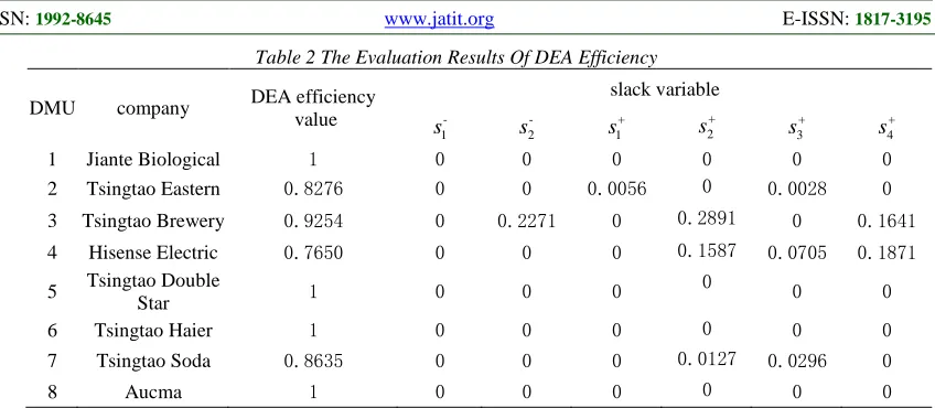
ISSN: 1992-8645 www.jatit.org E-ISSN: 1817-3195 Table 2 The Evaluation Results Of DEA Efficiency

DMU company DEA efficiency _value slack variable

-1

s

-2

s +

1

s s₂+ +

3

s +

4

s

1 Jiante Biological 1 0 0 0 0 0 0

2 Tsingtao Eastern 0.8276 0 0 0.0056 0 0.0028 0 3 Tsingtao Brewery 0.9254 0 0.2271 0 0.2891 0 0.1641 4 Hisense Electric 0.7650 0 0 0 0.1587 0.0705 0.1871

5 Tsingtao Double _Star 1 0 0 0 0 0 0

6 Tsingtao Haier 1 0 0 0 0 0 0

7 Tsingtao Soda 0.8635 0 0 0 0.0127 0.0296 0

8 Aucma 1 0 0 0 0 0 0

Table 3 shows that DEA efficiency values of Jiante Biological, Tsingtao Double Star, Tsingtao Haier and Aucma are all equal to 1. At least they are DEA grey weakly efficient. Furthermore, the slack variable s- and +

s are equal to 0. It indicates that the production and operation of the four listed companies are relative grey efficiency. The DEA efficiency values of other listed companies are all less than 1. It indicates that the other companies are DEA grey not weakly effective, less DEA grey effective.

6. CONCLUSION

In this paper, the grey system theory and DEA are combined to establish a new grey DEA model. The intersection of two different theories contributes to the development of the two disciplines theory. It provides a new perspective and an integrated approach to solve practical problems. We explore the deficiencies of grey system theory and DEA and integrate the advantages of the two theories. At last, we create a combination model. Our method has a more widely

applications. It not only improves grey

comprehensive evaluation method, but also enhances the grey comprehensive evaluation method holistic and systematic evaluation. It provides effective ideas and approaches. The study of this problem will improve the further integration and development of the grey comprehensive evaluation method and DEA method. It can provide more effective information for decision-makers. But it is just an attempt to form a new model by combining the two theories. There are more research need to further develop for inspection, correction and additional in practical applications. The problems need to be further studied are as follow. When the variable is a grey number, what is

the path of decision-making unit promoted to DEA efficient from a non-DEA effective? If it is scale effective when it is effective technology? How to achieve scale effective? Solving these problems will procure DEA model to explain the reality more effective.

ACKNOWLEDGEMENTS

This work was supported in part by the National Natural Science Foundation (70701017) and Natural Science Research Project of Henan Province Department of Education (2011A110002).

REFERENCES:

[1] ChangYung Kung, KunLi Wen.

“

Applying

Grey Relational Analysis and Grey Decision-Making to evaluate the relationship between company attributes and its financial performance---A case study of venture capital

enterprises in Taiwan

”,

Decision Support

Systems, Vol. 43, No. 3, 2007, pp. 842-852. [2] YiChung Hu.

“

Grey relational analysis and

radial basis function network for determining

costs in learning sequences

”,

Applied

Mathematics and Computation, Vol. 184, No. 2, 2007, pp. 291-299.

(6)

[4] A.J.C. Trappey, T.A. Chiang.

“

A DEA bench marking methodology for project planning and Management of new product development under decentralized profit-center business model

”

, Advanced Engineering Informations, Vol. 22, No. 4, 2008, pp. 1-7.

[5] Alex M.Andrew, “Grey Game Theory and Its Applications in Economic Decision-Making”,

Kybernetics, Vol. 39, No. 7, 2010, pp. 1205-1207.

[6] Li Qiaoxing, Liu Sifeng.

“

The Grey

Input-Occupancy-Output Analysis

”,

Kybernetics, Vol. 38, No. 4, 2009, pp. 306-313.

[7] QiaoXing Li.

“

Grey dynamic input-output

analysis

”,

Journal of Mathematical Analysis and Applications, Vol. 359, No. 2, 2009, pp. 514-526.

[8] Zhijie Chen, Qile Chen, Weizhen Chen, etc.

Inverse optimization for linearly constrained convex

separable programming problems

”,

European Journal of Operational Research,

Vol. 200, No.3, 2010, pp. 671-679.

[12] C.Yang, J.Zhang.

“

Two general methods for

inverse optimization problems

”,

Applied

Mathematics Letters, Vol. 112, No. 2, 1999, pp. 69-72.

[13] Andras Farago,Aron Szentesi, Balazs

Szviatovszki.

“

Inverse optimization in

high-speed networks

”,

Discrete Applied

Mathematics, Vol. 129, No.1, 2003, pp. 83-98.

[14] Ravindra K.Ahuja, James B.Orlin.

“

A Faster Algorithm for the Inverse Spanning Tree Problem

”,

Journal of Algorithms, Vol. 34, No. 1, 2000, pp. 177-193.

[15] L.M.Zerafat Angiz, A.Emrouznejad,

A.Mustafa, etal.

“

Selecting the most

preferable alternatives in a group decision

making problem using DEA

”,

Expert Systems

with Applications, Vol. 36, No. 5, 2009, pp. 9599-9602.

[16] R.Anderson, T.U.Daim, J.Kim.T

“

echnology

forecasting for wireless communication

” ,

Technovation, Vol. 28, No. 9, 2008, pp. 602-614.