On Crowd Density Estimation for Surveillance
H. Rahmalan, M.S. Nixon, J. N. Carter
University of Southampton, United Kingdom {hbr03r, msn, jnc}@ecs.soton.ac.uk
Keywords: Crowd Density, Translation Invariant
Orthonormal Chebyshev Moments, Minkowski Fractal Dimension, Grey Level Dependency Matrix
Abstract
The goal of this work is to use computer vision to measure crowd density in outdoor scenes. Crowd density estimation is an important task in crowd monitoring. The assessment is carried out using images of a graduation scene which illustrated variation of illumination due to textured brick surface, clothing and changes of weather. Image features were extracted using Grey Level Dependency Matrix, Minkowski Fractal Dimension and a new method called Translation Invariant Orthonormal Chebyshev Moments. The features were then classified into a range of density by using a Self Organizing Map. Three different techniques were used and a comparison on the classification results investigates the best performance for measuring crowd density by vision.
1 Introduction
Safety at venues, in particular stadiums or other large scale locations, where crowds tend to appear can be a critical business consideration. This is suited to surveillance systems using Closed Circuit Television (CCTV) where particular objects and their behaviour can be monitored through a long period of time. However, a human observer might miss some information because monitoring crowds through CCTV is very laborious and cannot be performed for all the cameras simultaneously [17]. Therefore, the use of automated techniques for monitoring crowds such as estimating a crowd’s density, tracking a crowd’s movement and observing a crowd’s behaviour, is necessary.
This paper focuses on crowd density estimation for several reasons. According to Au et al. [19], one of the key aspects in developing and maintaining a crowd safety system is to identify areas where crowds build up. Areas where crowds are likely to build up should be identified prior to the event or operation of the venue. This is important as crowds usually exist in certain areas or at particular times of the day. Areas where people are likely to congregate need careful observation to ensure crowd safety. Therefore, estimating crowd density may be a good solution for maintaining the crowds’ safety.
Estimating a crowd’s density is also used for management and control. However, this can became more difficult when the subjects in the crowd are self-occluding [1]. Thus, this has become of interest to researchers to develop a solution to estimate the crowd’s density. Generally, there are two main targets when estimating crowd’s density: 1) providing an approximate number of how many people are in the target scene [16, 1, 18, 5, 13]; and 2) providing a range of people in the crowd i.e. determining the density in broad classes [2, 3, 4]. The second target has been selected since it is more appropriate to general use.
In this paper, we develop three different techniques for estimating a crowd’s density in outdoor scenes. The difficulties in using outdoor scenes as input data include variation of illumination from weather and clothes, and also the floor surface texture. Two best methods from the previous work by Marana [2, 3, 4] have been chosen because they have previously demonstrated classification capability in indoor scenes. A new algorithm was also chosen using Chebyshev moments to extract the features for subsequent classification. The results from the three different algorithms will be compared to determine which is the most effective in estimating crowd density in outdoor scenes.
2 Methodology
This section describes three different methods that were used as the feature extractor: the Grey Level Dependency Matrix (henceforth GLDM)[2, 3], Minkowski Fractal Dimension (henceforth MFD)[3, 4] and our new method, Translation Invariant Orthonormal Chebyshev Moments (henceforth TIOCM). The GLDM and MFD were chosen as they have previously been observed to be able to provide good classification results.
2.1 Grey Level Dependency Matrix
The Grey Level Dependency Matrix (GLDM) was originally used in [12] to measure texture in satellite imagery, and in aerial and microscopic imagery. GLDM is also known as spatial grey level dependency matrix, grey level co-occurrence matrix or grey tone dependence matrix [12, 2].
In general, GLDM can be thought of as second-order joint conditional probability density functions, f(i,j|d,) which
calculate the probability of the pair of grey levels (i,j)
45o,90o, 135o and
Gis the number of grey levels of the image.
Four measurements [12, 2] to describe the GLDM will be used: the Contrast C, the Homogeneity H, the Energy Eg and
the Entropy Et.
1 1
2 0 0
, - , ,
G G
i j
C d i j f i j d
(1)
1 1 2 0 0 , , , 1 -G G i jf i j d H d i j
(2)
1 1
20 0
, , ,
G G i j
Eg d f i j d
(3)
1 1
0 0
, G G , , log , , i j
Et d f i j d f i j d
(4)In total, 16 features will be produced by the GLDM method for a moving window of size 20 x 20 sub-images with an interval of 10. Since the original picture is 200 pixels squared, 361 sets of features are generated per image.
2.2 Minkowski Fractal Dimension (MFD)
Fractals have been widely used for various problems in image processing, image analysis, vision and pattern recognition. Generally, the fractal dimension is a measurement of roughness of a shape [11]. The advantage of choosing the MFD as the feature extractor is that it allows the estimation of the fractal dimension of a region and so can be used as fractal texture measure.
The Minkowski sausages method is a straightforward technique to calculate an area’s influence by dilating a binary shape by a disk of diameter D[8]. For a single point the area
of interest grows continually, however it tends to fill any holes in dense shapes so that it looks like a nearly filled region, growing more slowly. This concept is similar to the box-counting approach. The fractal dimension is obtained by analysing the log-log plot of the area of influence versus D,
where curves with higher slopes are obtained for simple shapes, and the Bouligand-Minkowsky [4] fractal dimension is defined as F = 2 -S, where Sis the slope of the log-log plot
[4] defined by the logarithm of the number of white pixels, A,
divided by the logarithm of the dilations size, r.
log( ) log( ) A S r (5)
The first step in applying the MFD is to generate a thresholded version of the edge detected version of each input image, to generate a binary image. Phase congruency [10] was chosen as the edge detector because it is an illumination and contrast invariant measure of feature significance. The threshold was set at the average value of the phase congruency of each image. Then, dilations with structuring elements of different sizes, ranging from 1 torwere applied
to each binary image. Each dilation image will estimate the
fractal dimension of the input image. F was used as the single
feature.
2.3 Invariant Orthonormal Chebyshev Moments
Moments are powerful statistical tools for pattern recognition [7] and are known as a global descriptor [9]. Mukundan[14] proposed a discrete orthogonal moment, the Chebyshev moment. The advantages of the discrete orthogonal moments compared to continuous orthogonal moments such as Legendre and Zernike moments, are that; 1) there is no requirement of numerical approximation; 2) the orthogonality property is satisfied and defined in the image coordinate space; and 3) the results of reconstruction are of improved quality.
However, the discrete orthogonal Chebyshev moments have numerical problems when the required moment order is large, due to the recursive nature of the polynomial evaluation. To solve this problem, Mukundan[15] proposed orthonormal Chebyshev moments where orthonormalization was used to reduce the numerical instability while computing high order moments, although the recurrence relations can still induce large errors as the moment order increases.
The discrete orthonormal Chebyshev moments of an order
m+n, with the size of NxN for an image f(i,j), is defined as:
1 1 0 0
, N N
mn m n
i j
T t i t j f i j
(6)and the scaled Chebyshev polynomials tm
i
, m=0,1...N-1 are
defined by using the following recurrence relation
1 1
2 1
3 2
m m m m
t i it i t i t i
(7) where
2 1 2 22
2 2 2
2 2
3 2 2
2 4 1
1 4 1
1 2 1 1
2 3
m
m N m
N m
m N m
m m N m
m m N m
(8)
With initial condition for the above recurrence relation as
1 2 0 1 23 2 1 1 t i N
i N t i N N (9)
1 1 0 0
, N N
mn m c n c
i j
T t i i t j j f i j
(10)and the scaled Chebyshev polynomials tm
q
, where
c
q i i and m=0,1...N-1 are defined using the following
recurrence relation
1 1
2 1
3 2
m m m m
t q qt q t q t q (11) with an initial conditions of the above recurrence relation such as
1 2 0 1 23 2 1 1 t q N
q N t q N N (12)
while 1, 2, 3remains the same as written in equation (8).
This formulation has been demonstrated numerically to be invariant under translation as shown in Table 2.1. The results were based on the images in Figure 2.1, where 2.1 (a) is a silhouette image and 2.1 (b) is the silhouette in (a) shifted to the right by 100 pixels.
C he by sh ev M om en ts M om en ts O rd er Original Image Translated Image
00 38.768 38.768
10 -6.3979 27.176
01 10.815 10.815
20 46.785 66.904
02 63.105 63.105
O rt ho no rm al
11 -1.0155 8.3504
00 38.768 38.768
10 -66.98 -66.98
01 -66.98 -66.98
20 174.99 174.99
02 189.11 189.11
O rt ho no rm al (M od if ie d)
11 116.49 116.49
Table 2.1: Comparison results between orthonormal Chebyshev moments and Translation Invariant orthonormal Chebyshev moments (modified).
Experimentally, binary images were generated as described in Section 2.2. Zero up to 2nd order moments were then calculated and used as feature vectors.
50 100 150 200 250 300350 400 50 100 150 200 250 300 350 400
50 100 150 200 250 300 350 400 50 100 150 200 250 300 350 400
[image:3.595.72.270.371.578.2](a) Original Image (b) Translated Image Figure 2.1: Image of Silhouettes.
2.4 Training and Self Organizing Maps (SOM)
The SOM classifier was proposed by Kohonen[20] as a technique to aid visualization and interpretation large and high-dimensional data sets, reducing them onto a much lower dimensional network in an orderly manner. Marana [2, 3, 4] used a SOM to classify the images of crowd density specified ranges, using it both to reduce the dimensionality of the GLDM and as a final classifier. We have chosen not to use other classifiers to maintain fidelity with his work.
A SOM contains a number of neurons which is represented by a d-dimensional weight vector {m}=[m1, m2... md] where d is
equal to the dimension of the input feature vector. First, the weight vectors are initialized with small random values. Then in each training step, a sample vector is chosen randomly from the input data x and a similarity measurement between it
and all weight vectors of the SOM map are calculated. The similarity measurement is usually defined by a distance measure such as Euclidean distance. Best matching unit (BMU), denoted as c represents as the greatest or closest
similarity with the input sample x and can be defined as
below;
║x–mc║ = mini{║x–mi║} (13)
where ║.║ is the distance measure.
After the BMU has been determined, the BMU and its’ neighbours were updated and moved towards the input vector in the input space according to equation (14) below;
mi (t+1) = mi (t)+(t)h ci [x(t)–mi(t)]} (14) where t denotes time, x(t) is an input vector taken randomly
from the input data at time t, hci is the neighbourhood kernel
around the BMU and (t) as a learning rate is a deceasing
function of time between [0,1]. Here, the neighbourhood kernel around the BMU is the Gaussian neighbourhood function, defined as:
2 2 exp 2 c i ci r r h t (15)
where rc is the location of unit c,riis the neighbourhood node location on the SOM map while 2 is the neighbourhood radius at time t.
In early stages of training, relatively large initial learning rate 0 and neighbourhood radius 2 are used. As the training progresses, the neighbourhood radius is decreased with time. In the beginning of the training stages, SOM learns to roughly cover the space, while in the later stages, SOM fine tunes to describe the local details. After training, the SOM map is then labelled.
[image:3.595.71.258.661.753.2]3 Data
The data used for this experiment is video recorded at an outdoor reception where people congregated at different times during one day, simulating a surveillance application. The data comprises a range of densities from very low to very high crowds density. Three different datasets, labelled morning data, afternoon data and combined data (a combination of morning and afternoon data) were used. Each dataset has 50 images of training data and 25 images of test data, with equal numbers of images from each class. Examples of images are shown in Figure 3.1.
Very
[image:4.595.53.289.229.288.2]Low Low Moderate High Very high Figure 3.1: Sample Image of Crowds at Differencing Density
Images were classified according to the scheme described by Polus [2, 6], and shown in Table 3.1. In order to perform a standard comparison with the automatic crowd estimation, the number of people in each image was counted manually. In determining this ground truth, a person was counted in whole or partial body could be determined in the original colour images.
Level of Service Range of Density (people/m2)
Range of People
Group
A: Free (normal )
flow < 0.5 < 7 Very Low
B: Restricted flow 0.5 – 0.80 7 – 10 Low C1: Dense flow 0.81 – 1.26 11 – 16 Moderate C2: Very Dense
flow 1.27 – 2.0 17 – 26 High
[image:4.595.310.539.259.410.2]D: Jammed > 2.0 > 27 Very High Table 3.1: Level of Service
Each original image was 720 x 576 pixels and images were recorded every 10 seconds. A 200 x 200 region of the picture was used, representing an area brick pavement approximately 13m2. Training and test sets were chosen at random after images had been manually classified. The scene was viewed from a third floor window and recording took place in the morning and afternoon on a day with mixed weather conditions.
4 Results and Discussion
This section describes results of experiments using three different datasets (recorded in the morning, recorded in the afternoon and combined) of images according to the techniques described in Section 2. As previously stated the images are outdoor images with variation of illumination due to weather, cloth, and textured surface floor.
The number of people in each image was first counted manually to provide a ground truth estimation. Then, the images were selected and randomly divided into training and testing data. For each technique the training data was used to train a SOM with 5 clusters, corresponding to the number of density classes, which was subsequently used to classify the test data.
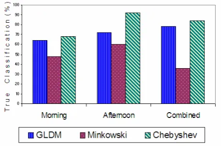
Figure 4.1 shows a graphical representation of the best results on test data, based on three different techniques according to three different datasets. Generally, the afternoon and combined data gives better results when compared to morning alone. This is because the afternoon data has smaller variation of illumination when compared with morning data.
Figure 4.1: Comparison classification for testing data of all datasets and all techniques
The results in Figure 4.1 show that both GLDM and Chebyshev methods out perform the fractal method, showing that on performance these experiments offer little to discriminate between them.
An investigation on why images were misclassified was carried out. There were two factors that influence the results to be misclassified. For example it was found that;
1) Shadow
The input data is an image of crowds outdoors where illumination due to sunshine may influence the object or cause the building to present shadows. Unfortunately, shadows can prove difficult to remove and could influence classification. This applies to all techniques.
2) Noise and clutter
[image:4.595.42.292.417.549.2]original image, followed by obtaining the edges using phase congruency in 4.2 (b). Here, it can be seen that the textured surface floor was also recognized and when binary images were generated, noise also appears. This process leads to misclassification.
ImT529000M.png Reduce Noise
a) Original Image c) After filter
Edge Detection
[image:5.595.72.269.150.467.2]b) After Phase Congruency Figure 4.2: Example of misclassification
To reduce the effects of the unwanted texture in MFD and TIOCM images, they were filtered with a 2D box function to remove isolated white points. Unfortunately, some information was been removed too. This led to additional misclassification and did not improve matters.
All algorithms were coded in MATLAB and used the Image and SOM toolboxes as required.
5 Conclusions
This paper presents three different ways to measure the crowd density in an outdoor scene by computer vision. Two methods, which are the Grey Level Dependency Matrix and the Minkowski Fractal Dimension, were used as they have previously shown good performance in classification. A new method, named as Translation Invariant Orthonormal Chebyshev Moments was also evaluated in this paper.
The images were taken during a graduation day ceremony. The number of people in the images was counted manually and then divided into three different test and training datasets, morning, afternoon and a combination of both. Each data contains a range of densities from very low to very high crowd density.
GLDM and TIOCM both out perform MFD under all conditions, however there was little to choose between them, given the small number of samples in this experiment. There is also some evidence that the GLDM requires almost an order of magnitude more time to classify a test image. If substantiated this would mandate the choice of TIOCM in practical situations.
Generally, the morning data gave worse results compared to afternoon and combined data. This is because the afternoon data has a much smaller variation of illumination compared with the morning data. Thus, we predict that the TIOCM, like GLDM may perform well when used for the estimation of crowd density for indoor scenes or other places where small variations of illumination appear.
It is clear that future evaluation is required, to determine how robust TIOCM is, especially when there are variations of the background.
Acknowledgements
One of the authors is grateful for the support of the Public Service Department of Malaysia and Kolej Universiti Teknikal Kebangsaan Malaysia for their financial support.
References
[1] A.C. Davies , J.H. Yin ,and S.A Velastin, “Crowd monitoring using image processing”, Electronics and
Communication Engineering Journal, volume 7, pp.
37-47, (1995).
[2] A. N. Marana, S. A. Velastin, L. F. Costa, and R. A. Lotufo, “Estimation of crowd density using image processing,” in Proc. IEE Colloquium Image Processing
for Security Applications, volume 11, pp. 1-8, (1997).
[3] A. N. Marana, S. A. Velastin, L. F. Costa, and R. A. Lotufo, “Automatic Estimation of Crowd Density using Texture”, Safety Science , volume 28, pp. 165 - 175,
(1998).
[4] A. N. Marana, L. da F. Costa, R. A. Lotufo, S. A. Velastin, “Estimating crowd density with Minkoski fractal dimension,” in Proc. Int. Conf. Acoust., Speech,
[5] D.B. Yang, H.H. Gonzalez-Banos, and L.J.Guibas , “Counting people in crowds with a real-time network of simple image sensors”, Proceedings. Ninth IEEE
International Conference on Computer Vision, volume
1, pp. 122 – 129, (2003)
[6] G.K. Still, “PhD Thesis : Crowd Dynamics”, Mathematics Department, Warwick University , (August, 2000).
[7] J. Zhang, and T. Tan, “Brief review of invariant texture analysis methods”, Pattern Recognition, Elsevier
Science Ltd., volume 35, No. 3, pp. 735 - 747, (2002).
[8] L.D.F Costa and R.M Cesar, “Shape Analysis and Classification, Theory and Practice”, CRC Press, (2000).
[9] M. S. Nixon and A. Aguado, “Feature Extraction and Image Processing”, Newnes, (2002).
[10] P. Kovesi, “Image Features from Phase Congruency”,
Videre: A Journal of Computer Vision Research,
volume 1, No. 3, pp.1-27, (1999)
[11] R. Fisher, K. Dawson-Howe, A. Fitzgibbon, C. Robertson, and E. Trucco, “Dictionary of Computer Vision and Image Processing” , Jon Wiley & Son Ltd , (2005).
[12] R.M. Haralick, “Statistical and structural approaches to texture”, Proceedings of the IEEE, volume 67, pp. 786
– 804, (1979)
[13] R. Ma, L. Li, W. Huang, and Q. Tian , “On pixel count based crowd density estimation for visual surveillance”,
IEEE Conference Cybernetics and Intelligent Systems,
volume 1, pp. 170 – 173, (2004)
[14] R. Mukundan, “Discrete Orthognal Moment Features Using Chebyshev Polynomials”, Proceedings of International. Conference on Image and Vision
Computing, pp. 20-25, (2000).
[15] R. Mukundan, “Improving Image Reconstruction Accuracy Using Discrete Orthonormal Moments
“,Proceedings of International. Conference On Imaging
Systems, Science and Technology, pp. 287-293, (2003)
[16] S.A. Velastin, J.H. Yin, A.C Davies, M.A Vicencio-Silva, R.E. Allsop, and A. Penn, “Analysis of crowd movements and densities in built-up environments using image processing”, Image Processing for Transport
Applications, IEE Colloquium, volume 8, pp. 1- 6,
(1993)
[17] S. Bouchafa, D. Aubert, and S. Bouza, “Crowd motion estimation and motionless detection in subway corridors by image processing” , (ITSC) Intelligent Transportation
System ,IEEE Conference, pp. 332 - 337, (1997).
[18] S.F. Lin, J.Y. Chen, and H. X. Chao, “Estimation of Number of People in Crowded Scenes Using Perspective Transformation,” in IEEE Trans. System, Man, and
Cybernetics, volume. 31, No. 6, pp. 645-654, (2001)
[19] S.Y.A. Au, M.C. Ryan, M.S. Carey, and S.P. Whalley, “Managing Crowd Safety in Public Venues: A Study to Generate Guidance For Venue Owners and Enforcing Authority Inspectors”, Health and Safety Executive , (1993).