M E T H O D
Open Access
OncoNEM: inferring tumor evolution
from single-cell sequencing data
Edith M. Ross and Florian Markowetz
*Abstract
Single-cell sequencing promises a high-resolution view of genetic heterogeneity and clonal evolution in cancer. However, methods to infer tumor evolution from single-cell sequencing data lag behind methods developed for bulk-sequencing data. Here, we present OncoNEM, a probabilistic method for inferring intra-tumor evolutionary lineage trees from somatic single nucleotide variants of single cells. OncoNEM identifies homogeneous cellular subpopulations and infers their genotypes as well as a tree describing their evolutionary relationships. In simulation studies, we assess OncoNEM’s robustness and benchmark its performance against competing methods. Finally, we show its applicability in case studies of muscle-invasive bladder cancer and essential thrombocythemia.
Keywords: Tumor evolution, Cancer evolution, Tumor heterogeneity, Single-cell sequencing, Phylogenetic tree
Background
Tumor development has long been recognized as an evo-lutionary process during which a cell population accu-mulates mutations over time and evolves into a mix of genetically distinct cell subpopulations, called clones [1]. The genetic intra-tumor heterogeneity that develops dur-ing clonal evolution poses a major challenge to cancer therapy, as it increases the chance of drug resistance and therefore treatment failure and relapse. Reliable methods for the inference of tumor life histories are important for cancer research, as they provide insights into ear-lier stages of cancer development and allow predictions about clinical outcome [2]. Furthermore, tumor life his-tories facilitate the discovery of mutations driving growth and resistance development, as well as the identification of unifying patterns of cancer evolution [3], thereby pro-viding an important stepping-stone towards enhanced treatment strategies for cancer. Inferring the evolutionary history of a tumor, however, remains challenging. Most methods developed for the inference of tumor evolution use data derived from bulk-sequencing of tumor samples, e.g., [4–6]. This approach requires deconvolution of the mixed signal of different tumor subpopulations, which is often ambiguous [7].
*Correspondence: [email protected]
Cancer Research UK Cambridge Institute, University of Cambridge, Robinson Way, Cambridge, UK
Challenges in single-cell sequencing
Recent advances in single-cell sequencing technologies have promised to reveal tumor heterogeneity at a much higher resolution [8–10]. However, single-cell sequencing comes with its own challenges.
The first challenge is noise in the observed genotypes, which includes false positive and false negative muta-tions as well as missing values. Reported false discov-ery rates vary from 2.67× 10⁻⁵ to 6.7× 10⁻⁵ [9–11], which means that false positives can easily outnumber true somatic variants [12]. The number of false positives is usually reduced by census-based variant calling, which only selects variants that are observed in multiple cells, but cannot remove sites of recurrent sequencing errors [13]. Reported allele dropout (ADO) rates vary from 0.16 to 0.43, yielding single nucleotide variant (SNV) data sets with large fractions of false negatives [9–11]. Related to this are missing values, which occur if all copies of a genetic locus fail to amplify, a very common problem in single-cell sequencing data sets [9–11]. Due to this noise, standard clustering methods often fail to identify sub-populations among the sequenced cells, turning even a seemingly simple task, such as mapping cells to clones, into a challenge.
The second challenge lies in unobserved subpopula-tions. Due to sampling biases, undersampling or extinc-tion of subpopulaextinc-tions, the sampled cells are likely to represent only a subset of the subpopulations that evolved
during the tumor’s life history. Thus, methods need to be able to infer unobserved ancestral subpopulations to retrace the evolution of a tumor accurately.
OncoNEM
Here, we describe OncoNEM (oncogenetic nested effects model), an automated method for reconstructing clonal lineage trees from somatic single nucleotide variants (SSNVs) of multiple single tumor cells that exploits the nested structure of mutation patterns of related cells.
OncoNEM probabilistically accounts for genotyping errors and tests for unobserved subpopulations, address-ing both of the challenges described above. It simulta-neously clusters cells with similar mutation patterns into subpopulations and infers relationships and genotypes of observed and unobserved subpopulations, yielding results that are more accurate than those of previous methods.
Existing methods
To gain insights into the evolutionary histories of tumors, various methods have been applied to single-cell data sets of somatic SNVs. Many studies use classic phylogenetic approaches. Examples include UPGMA used by Yu et al. [14] and neighbor joining used by Xu et al. [9], which are both closely related to hierarchical clustering. Hughes et al. [15] used neighbor joining trees as input for a like-lihood optimization method, which is based on a general time-reversible substitution model. Another classic phy-logenetic approach is Bayesian phyphy-logenetic inference as used by Eirew et al. [16]. None of these methods model the noise of single-cell data sets or infer trees based on subpopulations of cells.
Other studies use non-traditional methods. Some meth-ods first cluster cells into subpopulations and then infer minimum spanning trees. Gawad et al. [17] do this using model-based clustering, whereas Yuan et al. [18] use k-means and hierarchical clustering. Another method is BitPhylogeny, which uses a tree structured mixture model [18]. While mixture models are widely used and valu-able, e.g., for inferring the clonal composition of bulk-sequenced samples [5, 6], they require large data sets in order to converge to an accurate representation of the underlying distributions. Current single-cell data sets in contrast are small, containing usually fewer than 100 cells [8–12, 14, 15, 19]. Kim and Simon [20] proposed a method for inferring mutation trees. These are trees in which each node corresponds to a mutation instead of a clone.
For completeness, we also mention approaches that are not applicable in our case, because they are not fully automated or use other types of single-cell data. Li et al. [11] and Melchor et al. [21] performed partially man-ual inference. Potter et al. [22] defined subpopulations by grouping cells with identical genotypes into clones and then applied a maximum parsimony approach. Their data
sets were derived by single-cell qPCR of a few genetic markers, whereas our study focuses on noisy single-cell data sets with hundreds of genetic markers. In these large data sets, the observed genotypes differ between any two cells and the method used by Potter et al. [22] is there-fore not applicable. Like some of the studies mentioned above, Navin et al. [8] and Wang et al. [19] used neighbor joining but applied it to single-cell copy-number profiles obtained by whole-genome sequencing. Chowdhury et al. [2, 23] used Steiner trees to infer phylogenies from single-cell copy number profiles obtained from fluorescent in situ hybridization. Their algorithms, however, only infer trees from low-dimensional genotype spaces.
Outline
In the following, we first explain how OncoNEM infers clonal lineage trees from noisy SSNVs of single cells. Then we assess the robustness of OncoNEM and compare its performance with that of competing methods, which were chosen to be a representative selection of the approaches mentioned above. Finally, we describe the results of apply-ing OncoNEM in two case studies: a data set containapply-ing 44 single tumor cells from a muscle-invasive bladder tran-sitional cell carcinoma and a data set containing 58 single tumor cells from an essential thrombocythemia.
Results and discussion
Inferring clonal evolution with OncoNEM
The inputs to OncoNEM are (1) a binary genotype matrix containing the observed genotypes of every cell at every SSNV locus and (2) the false positive rate (FPR)αand false negative rate (FNR)β, which can be estimated from data (see ‘Materials and methods’).
The OncoNEM output includes (1) inferred tumor sub-populations, (2) a tree describing evolutionary relation-ships between these subpopulations and (3) posterior probabilities of the occurrence of mutations.
The OncoNEM algorithm consists of two main parts: (1) a probabilistic score that models the accumulation of mutations by noisy subset relations and (2) a sequence of inference algorithms to search for high-scoring models in the space of possible tree structures.
Probabilistic score for accumulation of mutations
OncoNEM predicts the expected mutation patterns based on the tree and then scores the fit between predicted and observed mutations patterns while probabilistically accounting for genotyping errors. A schematic illustra-tion of the OncoNEM scoring model is shown in Fig. 1. The derivation of the scoring function is described in ‘Materials and methods’.
Searching the tree space for high-scoring models
OncoNEM inference is a three-step process. We start with an initial search, where we restrict the model space to cell lineage trees. This yields a first estimate of the tree and its likelihood. The second step tests whether adding unobserved clones to the tree substantially increases the likelihood. The third step yields the final model of the clonal lineage tree by clustering cells within the previously derived tree into clones. An overview of the inference steps is shown in Fig. 2 and details are described in ‘Materials and methods’.
Simulation studies
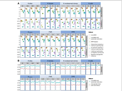
We performed comprehensive simulations to assess the robustness of OncoNEM to errors in the parameter esti-mates, and compared its performance to six baseline methods. As representatives of classic phylogenetic meth-ods we used likelihood optimization of neighbor joining trees, as applied by Hughes et al. [15], and Bayesian phy-logenetic inference, as used by Eirew et al. [16]. Both methods yield solutions where each cell corresponds to a different leaf in the tree. This type of tree is not directly comparable to the simulated one. To at least be able to evaluate the clustering solutions of the two methods, we identified subpopulations of cells within these trees by hierarchical clustering of the trees’ distance matrices with silhouette-score-based model selection. As represen-tatives of hierarchical clustering based methods and the
approaches used by Gawad et al. [17] and Yuan et al. [18], we used hierarchical and k-centroids clustering with silhouette-score-based model selection and subsequent minimum spanning tree construction. Furthermore, we compared our method to BitPhylogeny [18] and a method for inferring oncogenetic trees by Kim and Simon [20].
For all but Kim and Simon’s method, clustering per-formance was assessed using the V-measure, whereas the overall tree reconstruction accuracy was measured using the pairwise cell shortest-path distance. Since Kim and Simon’s method neither infers the position of the sequenced cells within the tree nor performs any clus-tering, V-measure and single-cell shortest-path distance cannot be used to assess its performance. Instead we calculated the accuracy of the inferred mutation orders. See ‘Materials and methods’ for details of benchmarking measures and data simulation.
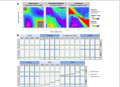
OncoNEM is robust to changes in error parametersαandβ To test if our method can infer the main model param-eters, FPRα and FNRβ, and to evaluate the robustness of our method to errors in those estimates, we simulated a tree containing ten clones, two of which were unob-served, with a total number of 20 cells. A corresponding genotype matrix with 200 SNVs was simulated using an FPR of 0.2, an FNR of 0.1 and 20 % missing values. Then, we inferred clonal lineage trees as described above, using various combinations of FNRs and FPRs, and compared the inferred trees to the ground truth. As Fig. 3a shows, a large range of parameter combinations yield solutions that are close to the original tree in terms of pairwise cell shortest-path distance and V-measure with both the inferred and the ground truth parameters lying in the mid-dle of this range. Similar results were obtained on a second data set that was simulated using a much lower FPR of 10−5 (see Additional file 1: Figure S1). These results
A B C D
[image:3.595.56.539.538.652.2]Fig. 2Toy example of OncoNEM inference steps. Given the observed genotypes and the input parametersαandβ, the log-likelihood of the start tree, which is by default a star-shaped tree, is−47.61. In the first step of the initial search, all neighbors of the star tree are scored. The highest scoring tree obtained in this step has a log-likelihood of−34.26. In this toy example, the highest scoring tree of the first step is also the best cell lineage tree, overall. Therefore, the initial search terminates with this tree as a solution. In the first refinement step, we find that inserting an unobserved node into the branch point of our current tree increases the log-likelihood by 3.82. Since this improvement is larger than the Bayes factor threshold of 2.3, the solution with the unobserved clone is accepted. In the final refinement step, cells are clustered along edges. In the toy example, only one clustering step does not decrease the log-likelihood by more than log()
demonstrate that OncoNEM is robust to changes in the model parameters.
OncoNEM estimates model parameters accurately
In the second simulation study, we further assessed the parameter estimation accuracy of OncoNEM. To generate different test data sets, we varied simulation parameters such as noise levels, number of cells, number of mutation sites, number of clones, fraction of missing values and the number of unobserved clones.
With unknown error rates, we compared the estimated FPR and FNR to the ground truth parameters. As shown in Fig. 3b, the estimated parameters are close to the ground truth parameters for all but the single-clone case. This demonstrates that OncoNEM estimates model parame-ters accurately over a wide range of simulation settings.
OncoNEM is robust to changes in
Next, we assessed the sensitivity of OncoNEM to changes in the Bayes factor threshold. We applied OncoNEM to each simulated data set described in the previous section, using varying values forand recoded the inferred num-ber of clones (see Fig. 4). In all simulation scenarios, the number of clones is largely independent of, unless this parameter is set to very low values ( <5). Throughout all further simulation and case studies,was kept constant at 10, which is well within the stable range.
OncoNEM outperforms baseline methods
Finally, using the same simulated data as above, we compared the performance of OncoNEM with known and unknown inference parameters to the performance of the six baseline methods mentioned above. The results of the method comparison are shown in Fig. 5. OncoNEM substantially outperforms the other methods for all simulation scenarios but the single-clone case.
It consistently yields results that have a smaller dis-tance to the ground truth and a higher V-measure than the baseline methods or, for oncogenetic trees, infers the order of mutation with a much higher accuracy. Overall, OncoNEM’s performance with unknown model parameters is comparable to its performance with given parameters.
In summary, the simulation results demonstrate that OncoNEM clearly outperforms the baseline methods for the tested simulation scenarios even if the model parame-ters are unknown a priori.
Case study 1: muscle-invasive bladder transitional cell carcinoma
We used OncoNEM to infer the evolutionary history of a muscle-invasive bladder transitional cell carcinoma previ-ously analyzed by Li et al. [11], who performed single-cell exome sequencing of 44 tumor cells, as well as exome sequencing of normal and tumor tissue. Li et al. esti-mated the average ADO rate to be 0.4 and the FDR to be 6.7×10⁻⁵. Using a census-filtering threshold of 3, they identified 443 SSNVs across the 44 cells. In their final genotype matrix, 55.2 % of the values were missing.
[image:4.595.57.541.86.212.2]50 100 200 300 1 5 10 20
0.01 0.08 0.15 0.22 0.29 0.36 0.43 0.50
0.01 0.08 0.15 0.22 0.29 0.36 0.43 0.50
1 2 3 4 10 20 30 50
# sites # clones # unobserved clones # cells
FPR
FNR
0.05 0.1 0.2 0.3 10-5 0.05 0.1 0.2 0.3 0.1 0.2 0.3 0.4
0.01 0.08 0.15 0.22 0.29 0.36 0.43 0.50
0.01 0.08 0.15 0.22 0.29 0.36 0.43 0.50
pmissing FNR FPR
FPR
FNR
Estimated value Ground truth Optimization grid
B
Parameter
Ground truth Estimate
Distance / V-measure
0 1
log(Bayes factor)
-1000 0
False positive rate
False negative rate
Bayes factor (compared to best model)
Normalized distance (to ground truth)
V-measure (relative to ground truth)
A
Fig. 3Parameter estimation.aDependence of OncoNEM results on inference parameters. Log Bayes factor of highest scoring model inferred with given parameter combination relative to highest scoring model overall. The inferred parameters (αˆ=0.22,βˆ=0.08) are close to the ground truth (α=0.2,β=0.1). A large range of parameter combinations around the ground truth parameters yield solutions close to the ground truth tree in terms of pairwise cell shortest-path distance and V-measure. The distance was normalized to the largest distance observed between any inferred tree and the ground truth.bParameter estimation accuracy. FPRs and FNRs estimated by OncoNEM for various simulation settings with five replicates each. Theblue linesmark the ground truth parameters. Thegrey linesmark the grid values over which FPR and FNR were optimized
Fig. 4Dependence of OncoNEM’s clustering solution on Bayes factor threshold. This figure shows the V-measure and the number of clones of the OncoNEM solution as a function offor various simulation scenarios. Everylinecorresponds to one data set of the method comparison study.Lines are color coded by parameter setting for the varied simulation parameter. In all simulation scenarios, the number of clones is largely independent of
[image:5.595.60.541.86.434.2] [image:5.595.66.541.559.673.2]A
B
Fig. 5OncoNEM performance assessment.aPerformance comparison of OncoNEM and five baseline methods. Shown are the distance and V-measure of inferred trees to ground truth. Results of single simulations are marked bydotsand colored by method, whileblack horizontal bars indicate the mean over five simulations for each method. The distances shown were normalized for the number of cellsnin the trees and were obtained by dividing the pairwise cell shortest-path distances byn(n−1)/2. Distances could only be calculated for three of the baseline methods. Values of the varied parameters are shown in thepanels at the top. As default parameters, we used an FNR of 0.1, an FPR of 0.2, 200 sites, ten clones, no unobserved clones, 20 cells and 20 % missing values.bPerformance comparison of OncoNEM and Kim and Simon’s oncogenetic tree method. Shown is the mutation order accuracy of the inferred trees for each of the simulated data sets. This measure is undefined for data sets without mutually exclusive mutations. Therefore, no values are shown for the single-clone case and the first replicate of the five-clone scenario, for which the simulated tree is linear
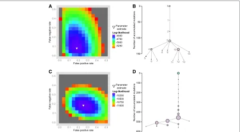
These results agree with the results of Li et al. who inferred three main subpopulations (A, B, C) with B and C having evolved from A. However, mapping the clone labels of Li et al. onto the OncoNEM tree shows that the assign-ment of cells to clones differs between the two approaches (see Additional file 1: Figure S2). Li et al. also inferred the origins of eight mutations in seven genes that are com-monly altered in muscle-invasive bladder transitional cell carcinomas. A comparison of their results with the pos-terior probability ofθ inferred by OncoNEM is shown in Table 1. The assignment of mutations to clones agrees in seven out of eight cases.
OncoNEM estimated the FPR to be 0.185 (see Fig. 6a). This error rate is higher than the expected value under the binomial model used for consensus
filtering by Li et al., which suggests that there might be recurrent sequencing errors in the data set. The FNR was estimated to be 0.08. This estimated value lies within the expected range of less than half the estimated ADO rate. See the parameter estimation section within ‘Materials and methods’ for an explana-tion of the conceptual differences between the original error rates estimated by Li et al. and the OncoNEM parameters.
[image:6.595.59.539.86.444.2]A B
C D
Fig. 6Case study results.a,bResults inferred by OncoNEM on bladder cancer data set. The estimated error rates areα=0.185 andβ=0.08. The inferred tree suggests a branching evolution with three major subpopulations.c,dResults inferred by OncoNEM on the essential thrombocythemia data set. The estimated error rates areα=0.255 andβ=0.185. The inferred tree suggests a largely linear evolution with some small
subpopulations branching off late during tumor evolution
Impact of loss of heterozygosity on inference results
The OncoNEM model assumes that mutations are never lost. Deletions that lead to loss of heterozygosity (LOH) are, however, common in various types of cancer.
We expect that our algorithm is able to infer good solutions despite LOH events, as long as the fraction of mutations affected by LOH is relatively small. In this
case, LOH-affected sites will simply contribute to the error rates of false positives and false negatives, depend-ing on whether the deletion occurred early or late after the original occurrence of the SNV.
[image:7.595.59.540.86.351.2]To support this claim, we identified the LOH-affected regions of the bladder cancer from a bulk-sequencing analysis by Li et al. (see Additional file 1: Table S1) and
Table 1Comparison of origin of mutations inferred by OncoNEM with origins inferred by Li et al.
1 2 3 4 5, 7 6 10 11, 12 13 8, 9, 14
A NIPBL 0.33 0.33 0.33 0.00 0.00 0.00 0.00 0.00 0.00 0.00
CFTR 0.45 0.45 0.09 0.00 0.00 0.00 0.00 0.00 0.00 0.00
DHX57 0.45 0.45 0.09 0.00 0.00 0.00 0.00 0.00 0.00 0.00
ASTN1 0.25 0.25 0.51 0.00 0.00 0.00 0.00 0.00 0.00 0.00
B ATM 0.00 0.00 0.00 1.00 0.00 0.00 0.00 0.00 0.00 0.00
C COL6A3 0.07 0.07 0.07 0.00 0.00 0.00 0.76 0.01 0.00 0.00
KIAA19581 0.00 0.00 0.00 0.00 0.00 0.00 0.98 0.00 0.00 0.00
KIAA19582 0.19 0.19 0.19 0.02 0.00 0.02 0.38 0.00 0.00 0.00
[image:7.595.57.540.571.697.2]removed all mutations within these regions from the mutation data set (6.3 % of all variant sites). We then applied OncoNEM to this reduced data set and compared the solution to the one obtained from the full data set. Additional file 1: Figure S4 shows that the inferred tree is largely stable and the overall tree structure remains the same.
Case study 2: essential thrombocythemia
In the second case study, we applied OncoNEM to a data set derived by single-cell exome sequencing of 58 single cells from an essential thrombocythemia [10]. Hou et al. estimated the average ADO rate to be 0.42 and the FDR to be 6.4×10⁻⁵. Using a census-filtering threshold of 5, they identified 712 SSNVs. Their final genotype matrix contained 57.7 % missing values.
The genotypes were binarized and OncoNEM was applied as in the previous case study. The inferred tree is shown in Fig. 6d. Again, the tree suggests that all tumor cells are descendants of a single founder cell. The majority of cells belong to subpopulations that are related through a linear trajectory. All detected branching events have occurred late during tumor development, i.e., after the tumor had already acquired more than 60 % of its mutations.
These results agree with the somatic mutant allele fre-quency spectrum analysis of Hou et al. that suggests that the neoplasm is of monoclonal origin [10], while Kim and Simon inferred a mutation tree with a complex hierarchy [20]. Using BitPhylogeny, Yuan et al. [18] inferred a poly-clonal origin. However, with 58 cells, the data set might be too small for their method to converge.
OncoNEM estimated the FPR and FNR to be 0.255 and 0.185, respectively. The FPR estimate is again higher than expected under the binomial model, whereas the FNR lies within the expected range. As in the previous case study, running OncoNEM with similar parameters yields similar trees (see Additional file 1: Figure S5).
Given the error rates inferred by OncoNEM, the log-likelihood of the BitPhylogeny tree computed under the OncoNEM model is−11584, whereas the OncoNEM tree has a log-likelihood of−9964. The fact that the OncoNEM solution has a much higher likelihood than the BitPhy-logeny tree shows that the differences are not due to the heuristic nature of OncoNEM’s search algorithm, but instead suggest that BitPhylogeny did not converge to the optimal solution.
These two case studies showed how OncoNEM can extend and improve on previous analyses of these data sets.
Conclusions
OncoNEM is an accurate probabilistic method for infer-ring intra-tumor phylogenies from noisy observations of SSNVs of single cells. It is based on the nested structure
of mutation patterns of phylogenetically related cells. The input to our method is a binary genotype matrix, which may contain missing values as well as false positives and false negatives. OncoNEM identifies subpopulations within a sample of single cells and estimates their evo-lutionary relationships and underlying genotypes, while accounting for the high error rates of single-cell sequenc-ing. OncoNEM can estimate model parameters directly from the input data and is robust to changes in those estimates.
In simulations, OncoNEM performs well for error rates of current single-cell data sets and large fractions of miss-ing values, and substantially outperforms baseline meth-ods. We have applied OncoNEM in two case studies, showing that the OncoNEM results agree with previous results, which were based on manual inference and the analysis of somatic mutant allele frequency spectra, while also providing a more refined picture of the tumors’ histo-ries. In one case study, we have also shown that OncoNEM yields robust results even if parts of the genome are affected by LOH.
Our general recommendation is to blacklist LOH-affected regions before OncoNEM inference, if additional data like bulk-sequencing is available. If the evolution of the tumor is known to be copy number driven and LOH affects very large parts of the genome, we recommend using a copy-number-based method for inferring tumor evolution.
OncoNEM can easily be applied to single-cell data sets of current size. For much larger data sets, the current search algorithm may become too computationally expen-sive. Currently the model cannot be used for copy number variations, which are not independent of each other and show horizontal dependencies [27] and we plan to extend the model to this data type in the future.
Recent advances have made it possible to sequence both the genome and transcriptome of a single cell [28, 29]. In the future, this will allow us to combine single-cell phy-logenies with single-cell transcriptomics to gain insights into how the expression of genes changes as a tumor evolves.
In summary, OncoNEM is a major step towards under-standing the clonal evolution of cancer at single-cell reso-lution.
Materials and methods Likelihood of a clonal lineage tree Data
sitel, where 0, 1 and NA encode an unmutated, mutated or unknown site, respectively.
Clonal lineage trees
We assume that a clonal lineage tree is a directed not necessarily binary tree T whose root is the unmutated normal. Every node of this tree represents a clone c ∈
{1,. . .,N}that contains 0, 1 or multiple cells of the data set. Letc(k)denote the clone that contains cellk. In the following, we assume without loss of generality that the root has index 1.
OncoNEM
An OncoNEM has two parts: the clonal lineage treeT and the occurrence parameter= {θl}ml=1, whereθltakes the valuecof the clone where mutationloriginated.
The core of our method is a function that defines the probability of the OncoNEM given a data set Dand is derived in the following. Using a Bayesian approach, the posterior probability ofT andgivenDcan be written as
P(T,|D)= P(D|T,)P(|T)P(T)
P(D) . (1)
The model priorP(T)can be used to incorporate prior biological knowledge. We assume it to be uniform over the search space. The normalizing factorP(D)is the same for all models and it is not necessary to compute it when comparing them. Therefore,
P(T,|D)∝P(D|T,)P(|T). (2)
Likelihood for known
Let us assume that we know for each locus l in which clone the mutation occurred and that no mutations occur in the normal. This is equivalent to restricting the param-eter space ofθlto{2,. . .,N}and is justified by stringent variant filtering of the input data.
GivenT and, we can predict the genotype of every cell: ifc is the clone in which a mutation occurred, the mutation is present in c and all descendants of c and absent in all other clones, i.e., given θl = c, the tree determines the predicted genotypeδkl.
Finally, to calculate the likelihood of(T,), we com-pare the expected genotypes with the observed ones. We model the genotyping procedure as draws of binary ran-dom variablesωkl from the sample space = {0, 1}and assume that, given T and , the random variables are independent and identically distributed according to the probability distribution
P(ωkl|δkl)=
P(0|0) P(1|0) P(0|1) P(1|1)
=
1−α α
β 1−β
,
(3)
whereαandβare global probabilities of false positive and false negative draws, respectively.
We interpret the observed genotypesdklas events from the event spaceP( )= {∅,{0},{1},{0, 1}}, where a miss-ing value corresponds to the event{0, 1}. Then, the prob-ability of the observed genotypes D given T and is
P(D|T,)= m l=1 n k=1
P(ωkl∈dkl|δkl), (4)
where
P(ωkl ∈dkl|δkl)=
⎧ ⎪ ⎪ ⎪ ⎪ ⎨ ⎪ ⎪ ⎪ ⎪ ⎩
1−α ifdkl = {0}andδkl =0
α ifdkl = {1}andδkl =0
β ifdkl = {0}andδkl =1 1−β ifdkl = {1}andδkl =1 1 ifdkl = {0, 1}
(5)
is the probability of a single observation given the pre-dicted genotype.
Likelihood for unknown
So far we assumedto be known, but this is generally not the case. To derive the likelihood of the entire data matrix, we treatas a nuisance parameter and marginal-ize over it. Furthermore, we make two assumptions: First, the occurrence of one mutation is independent of the occurrence of all other mutations, i.e.,
P(|T)= m
l=1
P(θl|T), (6)
and second, the prior probability of a mutation occurring in a clone is
P(θl=c|T)=
0 ifcis the normal(c=1), 1
N−1 otherwise.
(7)
Then the marginal likelihood is
P(D|T)=
P(D|T,)P(|T)d
= 1
(N−1)m m l=1 N c=2 n k=1
P(ωkl ∈dkl|T,θl=c)
=( 1
N−1)m m l=1 N c=2 n k=1
P(ωkl ∈dkl|δkl).
(8)
Algorithms to infer OncoNEMs
OncoNEM inference is a three-step process of initial search, testing for unobserved clones and clustering.
Step 1. Initial search: building a cell tree
infea-sible for trees with more than nine nodes. Therefore, we implemented a heuristic local search (see Algorithm 1), which avoids getting trapped in local optima by returning to neighbors of high-scoring previous solutions.
Step 2. Refinement: testing for unobserved clones
The number of sequenced single cells is usually small compared to the tumor size. Consequently, some clones of the tumor may not be represented in the single-cell sample. This problem is similar to the ‘unknown unknowns’ problem in reconstructing biological pathways [30], where latent variables that cause additional patterns in the observed data set can be inferred. In the OncoNEM setting, unobserved clones with at least two child clones create additional mutation patterns and can, therefore, potentially be inferred. OncoNEM accounts for this pos-sibility by testing if there is a lineage tree with additional, unobserved branch nodes that can better explain the observed data (see Algorithm 2). Unobserved clones that linearly connect observed clones cannot be inferred, but they also do not change the shape of the tree.
Briefly, the algorithm generates trees withn+1 nodes from the previous solution by inserting an unobserved node into its branch points. These trees are used as start trees in a new search that optimizes the position of the unobserved node in the tree. A larger model is accepted if the Bayes factor of the larger versus the smaller model is larger than a threshold (see below). If the larger model passes the threshold, these expansion steps are repeated, otherwise the algorithm terminates with the smaller solution.
Step 3. Refinement: clustering cells into clones
The clustering procedure tests if the data can be explained better or equally well by a clonal lineage tree in which mul-tiple cells correspond to the same node (see Algorithm 3). Nodes are clustered iteratively along branches until merg-ing cells into clones decreases the likelihood by more than a factor of 1/ compared to the best clustering solution found so far. Cells may be clustered into clones because they are genetically very similar or because of the lim-ited information content of the data, which can be due to genotyping errors, missing values or a restricted number of SSNVs in the sequenced regions of the genome.
Choosing the Bayes factor threshold
Choosing the parameteris a trade-off between declaring clones with little support from the data and overly strict clustering. In this setting, choosing >1 means that we prefer the smaller model unless the strength of evidence for the larger model compared to the smaller one exceeds a certain threshold. Jeffreys’s [31] or Kass and Raftery’s [32] scale for the interpretation of the Bayes factor can be used as guidance. We used a value of = 10, which denotes strong evidence according to Jeffreys’s scale.
Algorithm 1: Heuristic search algorithm. D is the genotype matrix, FPR and FNR are the error rates and startTrees is the list of trees the heuristic search is started from. The algorithm terminates if the highest scoring solution has not changed for more thanδiterations. We define the neighbors of a given tree as all trees that can be generated from the current tree by assigning a new parent to one of the nodes or by swapping two nodes that are connected by an edge. For the initial search, the start tree has a star topology
1 FunctionheuristicSearch(D, FPR, FNR, startTrees,δ)
2 initializeconsideredTrees←empty;
/* List of all scored trees,
ordered by likelihood */
3 initializepriorityQueue←empty;
/* List of all trees that have been scored themselves and whose neighbors have not yet been scored explicitly, ordered
by likelihood */
4 initializecounter←0;
/* Counts search steps since last change of highest scoring
solution */
5 fortreeinstartTreesdo 6 score tree;
7 add tree to consideredTrees; 8 add tree to priorityQueue;
9 end
10 bestTree←consideredTrees[1]; 11 whilecounter≤δdo
12 currentTree←priorityQueue[1]; 13 delete currentTree from priorityQueue; 14 forevery neighbor of currentTreedo 15 ifneighbor∈/consideredTreesthen
16 score neighbor;
17 add neighbor to consideredTrees;
18 add neighbor to priorityQueue;
19 end
20 end
21 ifbestTree=consideredTrees[1]then
22 counter←0 ; /* Highest scoring
solution changed */
23 bestTree←consideredTrees[1];
24 else
25 counter←counter +1;
26 end
27 end
28 returnconsideredTrees
Algorithm 2:Expansion algorithm−tests for unob-served clones.Tnrepresents the cell lineage tree withn nodes inferred by the initialheuristicSearch()
andis the Bayes factor threshold
1 FunctionexpandTree(Tn,) 2 initializei←0;
3 repeat 4 i←i+1;
5 /* Generate start trees */
startTrees←star tree withn+inodes; 6 forevery node inTn+i−1that has at least two
childrendo
7 Generate a new tree by inserting an unobserved node into the branch point; 8 Add tree to startTrees;
9 end
10 consideredTrees←
heuristicSearch(startTrees);
11 Tn+i←highest scoring tree in
consideredTrees in which every unobserved node has at least two children;
12 K←P(D|Tn+i)/P(D|Tn+i−1);/* Calculate
Bayes factor */
13 untilK< ; 14 returnTn+i−1
15 end
Estimating, the occurrence of mutations
Given a lineage tree, we can estimate which clones acquired which mutations during tumor development. To do this, we calculate the posterior probability of a muta-tion having occurred in clonec. Using a uniform prior for the occurrence parameterθl ∈ {2,. . .,N}, we obtain
P(θl=c|T,D)= 1 Z
n
k=1
P(ωkl ∈dkl|T,θl=c), (9)
with normalizing constant
Z= N
c=2 n
k=1
P(ωkl ∈dkl|T,θl=c). (10)
The branch lengthsL of the tree can be estimated as the expected number of mutations that separate a clonec from its parent pa(c),
Lpa(c),c= m
l=1
P(θl =c|T,D). (11)
Estimating model parametersαandβ
Previous studies have estimated FDRs and ADO rates from the sequencing data [9, 10]. These error rates are, however, not equivalent to the error parameters FPR α
Algorithm 3:Clustering algorithm.T represents the cell lineage tree inferred byexpandTree()andis the Bayes factor threshold
1 FunctionclusterTree(Tstart,)
2 initializeT ←Tstart; /* Current tree */
3 initializeT∗←Tstart;/* Best tree scored
so far */
4 repeat
5 forevery edge eido
6 Generate clustered treeTeifromT by
merging the clones connected byei;
7 end
8 Te∗
i ←arg max
Tei P(D|Tei);
9 K←P(D|T∗)/P(D|Te∗
i);
10 ifK≤then 11 T ←Te∗
i ; /* Accept clustering
solution */
12 ifP(D|T∗) <P(D|Te∗
i)then
13 T∗←Te∗
i ;/* Save clustering
solution as new best tree */
14 end
15 end
16 untilK> ; 17 returnT
18 end
and FNRβ used by OncoNEM. This is due to three pre-processing steps that are applied to the sequencing data to generate the final genotype matrix.
In the first step, only sites that appear to be mutated are selected. Selecting only sites that report mutations from all sequenced sites enriches for false positives. It also means that the FPR used by OncoNEM is conceptu-ally very different from the FDR reported in these studies. The FPR describes what fraction of truly non-mutant sites is reported as mutant in the observed genotype matrix, whereas the FDR corresponds to the number of false positive variants per sequenced base pair.
Thirdly, a binarization step is performed that inter-prets all homozygous mutant sites as heterozygous nor-mal/mutant. This step reduces the FNR by approximately 50 % and further explains why the FDR is expected to differ from previously estimated ADO rates.
While all of these steps are expected to change the error rates of the final data set, the exact impact on the parameters is difficult to estimate. Therefore, we chose to estimate error rates for our model directly from the data.
We treat the selection of model parameters as part of the learning problem and estimate them using a maximum likelihood approach, similar to Zeller et al. [33]. We create a grid of parameter combinationsα andβ and optimize
T given these parameters using the heuristic search algo-rithm. Then, we choose the parameter combination that yields the highest scoring tree and infer a clonal lineage tree as described above.
This parameter estimation process is computationally expensive compared to the tree inference. However, it can easily be parallelized and the grid of parameter combina-tions can be coarse as OncoNEM is robust to changes in the model parameters around the optimum (see simula-tion results). Furthermore, the range of tested parameter combinations can be reduced in the presence of prior knowledge.
Data simulation
For the simulation study, data sets were created in a two-step procedure that consists of (1) generating a tree structure and (2) simulating the corresponding genotypes.
Simulating clonal lineage trees
To simulate a tree with cclones, we select clone one to be the root and the parent of the second clone. Then, the remaining clones are added iteratively by choosing a non-root node that is already part of the tree with uniform probability as parent.
When simulating trees with unobserved clones, we count how many nodes in the simulated tree have at least two children. If this number is greater than or equal to the desired number of unobserved clonescu, we randomly choose cu of these nodes as unobserved clones, other-wise a new tree is simulated. Next, we assign one cell to every observed clone. For the remaining cells, clones are chosen iteratively with a probability proportional to the current clone size, to generate clones of different sizes.
Simulating genotype observations
For every mutation site, we choose the occurrence param-eterθlwith uniform probability from all non-root nodes. Given and the tree structure, the full matrix of true genotypes is obtained by setting an entry to 1, if the muta-tion occurred in a clone that is ancestral to the cell’s clone
or if the mutation occurred in the clone containing the cell itself, and 0 otherwise.
Observed genotypes are derived from true genotypes by (1) setting a fractionpmissing of randomly chosen values to NA, (2) setting a fractionαof unmutated, non-missing entries to 1 and (3) setting a fraction β of mutated, non-missing entries to 0. If this yields sites without any observed mutations, we add, for each of these sites, a false positive to a randomly chosen cell. Finally, to avoid a bias in the method testing, we randomize the order of cells in the matrix of observed genotypes.
Comparison measures for method benchmarking
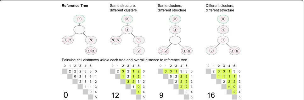
Clustering performance was assessed using the V-measure [34], an entropy-based cluster evaluation mea-sure that assesses both completeness and homogeneity of the clustering solution. The V-measure takes values from 0 to 1, with higher values indicating a better performance. To assess the similarity between trees, we developed a distance measure called pairwise cell shortest-path dis-tance(see Fig. 7). Given are two trees,T1andT2, built on the same set of cells{1,. . .,n}, but potentially differing in the number of nodes (clones). Note that the root of a tree can be an empty node. To ensure that every node of the tree is taken into account in the distance measure, we add an extra cell to the root before calculating the distance. Without loss of generality, we denote this additional cell in the root node with index 0. For every pair of cellsiandj, we compute the shortest-pathdij(·)between the two cells in each tree. If the two cells belong to the same clone, their shortest-path distance is 0, otherwise the shortest-path distance equals the number of edges (regardless of direc-tion) that separate the clones of the two cells. Finally, we sum up the absolute differences between the shortest-path distances of all unordered pairs of cells in the two trees to obtain the overall pairwise cell shortest-path distance:
d(T1,T2)= n−1
i=0 n
j=i+1
|dij(T1)−dij(T2)|. (12)
A proof that this distance is a metric can be found in Additional file 1.
We define themutation order accuracyof a treeT1given the ground truth treeT2as the average of
• the fraction of correctly inferred pairwise mutation orders, i.e., the probability that mutation a is
upstream of mutation b inT1given that a is upstream of b inT2, and
• the fraction of correctly inferred mutually exclusive mutations, i.e., the probability that two mutations a and b lie on separate branches inT1given that a and b lie on separate branches inT2
Fig. 7Comparing clonal trees with the pairwise cell shortest-path distance. Theyellowentries in the pairwise distance matrices indicate differences from the reference tree
Software and data availability
OncoNEM has been implemented in R [35] and is freely available under a GPL3 license on bitbucket [36]. Additional file 2 is a Knitr file reproducing all figures of the simulation studies. Additional file 3 is a Knitr file repro-ducing all figures of the case studies. Additional files 4 and 5 are the corresponding PDF files.
The processed single-cell data sets are provided in the OncoNEM R package. The sequencing data from both single-cell studies are deposited in the NCBI Sequence Read Archive [37]. The accession numbers are [SRA:SRA051489] for the bladder cancer study [11] and [SRA:SRA050202] for the essential thrombocythemia study [10].
Ethics approval
Ethics approval was not needed for this study.
Additional files
Additional file1:Supplementary information. A PDF file containing five supplementary figures, one supplementary table, the definition of the pairwise cell shortest-path distance and a proof showing that this distance is a metric. (PDF 631 kb)
Additional file 2:Knitr file for simulation studies. An rnw file for repro-ducing the results of the simulation studies. (RNW 58.3 kb)
Additional file 3:Knitr file for case studies. An rnw file for reproducing the results of the case studies. (RNW 27.7 kb)
Additional file 4:PDF of compiled knitr script for simulation studies. A PDF file reproducing the results of the simulation studies. (PDF 594 kb) Additional file 5:PDF of compiled knitr script for case studies. A PDF file reproducing the results of the case studies. (PDF 463 kb)
Abbreviations
ADO, allele dropout; FNR, false negative rate; FPR, false positive rate; LOH, loss of heterozygosity; SNV, single nucleotide variant; SSNV, somatic single nucleotide variant.
Competing interests
The authors declare that they have no competing interests.
Authors’ contributions
FM planned and outlined the study. EMR developed and implemented the model and simulated and analyzed the data. EMR and FM wrote the manuscript. All authors read and approved the final manuscript.
Acknowledgments
The authors would like to acknowledge the support of the University of Cambridge, Cancer Research UK and Hutchison Whampoa Limited.
Funding
This work was funded by CRUK core grant C14303/A17197.
Received: 29 March 2016 Accepted: 30 March 2016
References
1. Nowell PC. The clonal evolution of tumor cell populations. Science. 1976;194(4260):23–8.
2. Chowdhury SA, Shackney SE, Heselmeyer-Haddad K, Ried T, Schäffer AA, Schwartz R. Phylogenetic analysis of multiprobe fluorescence in situ hybridization data from tumor cell populations. Bioinformatics. 2013;29(13):189–98. doi:10.1093/bioinformatics/btt205.
3. Sidow A, Spies N. Concepts in solid tumor evolution. Trends Genet. 2015;31(4):208–14. doi:10.1016/j.tig.2015.02.001.
4. Nik-Zainal S, Van Loo P, Wedge DC, Alexandrov LB, Greenman CD, Lau KW, et al. The life history of 21 breast cancers. Cell. 2012;149(5):994–1007. doi:10.1016/j.cell.2012.04.023.
5. Oesper L, Mahmoody A, Raphael BJ. THetA: inferring intra-tumor heterogeneity from high- throughput DNA sequencing data. Genome Biol. 2013;14:. doi:10.1186/gb-2013-14-7-r80.
6. Roth A, Khattra J, Yap D, Wan A, Laks E, Biele J, et al. PyClone: statistical inference of clonal population structure in cancer. Nat Methods. 2014;11(4):396–8. doi:10.1038/nmeth.2883.
7. Jiao W, Vembu S, Deshwar AG, Stein L, Morris Q. Inferring clonal evolution of tumors from single nucleotide somatic mutations. BMC Bioinform. 2014;15:35. doi:10.1186/1471-2105-15-35.
8. Navin N, Kendall J, Troge J, Andrews P, Rodgers L, McIndoo J, et al. Tumour evolution inferred by single-cell sequencing. Nature. 2011;472(7341):90–4. doi:10.1038/nature09807.
9. Xu X, Hou Y, Yin X, Bao L, Tang A, Song L, et al. Single-cell exome sequencing reveals single-nucleotide mutation characteristics of a kidney tumor. Cell. 2012;148(5):886–95. doi:10.1016/j.cell.2012.02.025.
10. Hou Y, Song L, Zhu P, Zhang B, Tao Y, Xu X, et al. Single-cell exome sequencing and monoclonal evolution of a JAK2-negative myeloproliferative neoplasm. Cell. 2012;148(5):873–85. doi:10.1016/j.cell.2012.02.028.
[image:13.595.58.541.87.247.2]muscle-invasive bladder cancer. GigaScience. 2012;1(1):12. doi:10.1186/2047-217X-1-12.
12. Lohr JG, Adalsteinsson VA, Cibulskis K, Choudhury AD, Rosenberg M, Cruz-Gordillo P, et al. Whole-exome sequencing of circulating tumor cells provides a window into metastatic prostate cancer. Nat Biotechnol. 2014;32(5):479–84. doi:10.1038/nbt.2892.
13. Navin NE. Cancer genomics: one cell at a time. Genome Biol. 2014;15(8): 452. doi:10.1186/s13059-014-0452-9.
14. Yu C, Yu J, Yao X, Wu WK, Lu Y, Tang S, et al. Discovery of biclonal origin and a novel oncogene SLC12A5 in colon cancer by single-cell
sequencing. Cell Res. 2014;24(6):701–12. doi:10.1038/cr.2014.43. 15. Hughes AE, Magrini V, Demeter R, Miller CA, Fulton R, Fulton LL, et al.
Clonal architecture of secondary acute myeloid leukemia defined by single-cell sequencing. PLoS Genet. 2014;10(7):1004462.
doi:10.1371/journal.pgen.1004462.
16. Eirew P, Steif A, Khattra J, Ha G, Yap D, Farahani H, et al. Dynamics of genomic clones in breast cancer patient xenografts at single-cell resolution. Nature. 2015;518(7539):422–6. doi:10.1038/nature13952. 17. Gawad C, Koh W, Quake SR. Dissecting the clonal origins of childhood
acute lymphoblastic leukemia by single-cell genomics. PNAS. 2014;111(50):17947–52. doi:10.1073/pnas.1420822111.
18. Yuan K, Sakoparnig T, Markowetz F, Beerenwinkel N. BitPhylogeny: a probabilistic framework for reconstructing intra-tumor phylogenies. Genome Biol. 2015;16(1):36. doi:10.1186/s13059-015-0592-6. 19. Wang Y, Waters J, Leung ML, Unruh A, Roh W, Shi X, et al. Clonal
evolution in breast cancer revealed by single nucleus genome sequencing. Nature. 2014;512(7513):155–60. doi:10.1038/nature1360. 20. Kim KI, Simon R. Using single cell sequencing data to model the
evolutionary history of a tumor. BMC Bioinform. 2014;15:. doi:10.1186/1471-2105-15-27.
21. Melchor L, Brioli A, Wardell CP, Murison A, Potter NE, Kaiser MF, et al. Single-cell genetic analysis reveals the composition of initiating clones and phylogenetic patterns of branching and parallel evolution in myeloma. Leukemia. 2014;28(8):1705–15. doi:10.1038/leu.2014.13. 22. Potter NE, Ermini L, Papaemmanuil E, Cazzaniga G, Vijayaraghavan G,
Titley I, et al. Single-cell mutational profiling and clonal phylogeny in cancer. Genome Res. 2013;23(12):2115–25. doi:10.1101/gr.159913.113. 23. Chowdhury SA, Shackney SE, Heselmeyer-Haddad K, Ried T, Schäffer AA,
Schwartz R. Algorithms to model single gene, single chromosome, and whole genome copy number changes jointly in tumor phylogenetics. PLoS Comput Biol. 2014;10(7):1003740. doi:10.1371/journal.pcbi.1003740. 24. Markowetz F, Bloch J, Spang R. Non-transcriptional pathway features
reconstructed from secondary effects of RNA interference. Bioinformatics. 2005;21(21):4026–32. doi:10.1093/bioinformatics/bti662.
25. Markowetz F, Kostka D, Troyanskaya OG, Spang R. Nested effects models for high-dimensional phenotyping screens. Bioinformatics. 2007;23(13): 305–12. doi:10.1093/bioinformatics/btm178.
26. Kimura M. The number of heterozygous nucleotide sites maintained in a finite population due to steady flux of mutations. Genetics. 1969;61(4):893. 27. Schwarz RF, Trinh A, Sipos B, Brenton JD, Goldman N, Markowetz F.
Phylogenetic quantification of intra-tumour heterogeneity. PLoS Comput Biol. 2014;4:1003535. doi:10.1371/journal.pcbi.1003535.
28. Dey SS, Kester L, Spanjaard B, Bienko M, van Oudenaarden A. Integrated genome and transcriptome sequencing of the same cell. Nat Biotechnol. 2015;33(3):285–9. doi:10.1038/nbt.3129.
29. Macaulay IC, Haerty W, Kumar P, Li YI, Hu TX, Teng MJ, et al. G&T-seq: parallel sequencing of single-cell genomes and transcriptomes. Nat Methods. 2015;12(6):519–22. doi:10.1038/nmeth.3370.
30. Sadeh MJ, Moffa G, Spang R. Considering unknown unknowns: reconstruction of nonconfoundable causal relations in biological networks. J Comput Biol. 2013;20(11):920–32. doi:10.1089/cmb.2013.0119. 31. Jeffreys H. Theory of Probability, 3rd ed. Oxford: Oxford University Press;
1998.
32. Kass RE, Raftery AE. Bayes factors. JASA. 1995;90(430):773–95. doi:10.1080/01621459.1995.10476572.
33. Zeller C, Frohlich H, Tresch A. A Bayesian network view on nested effects models. EURASIP J Bioinform Syst Biol. 2009;1:195272.
doi:10.1155/2009/195272.
34. Rosenberg A, Hirschberg J. V-measure: a conditional entropy-based external cluster evaluation measure. In: Proceedings of the 2007 Joint Conference on Empirical Methods in Natural Language Processing and
Computational Natural Language Learning (EMNLP-CoNLL). Prague, Czech Republic: Association for Computational Linguistics; 2007. p. 410–20.
35. R Core Team. R: a language and environment for statistical computing. Vienna: R Foundation for Statistical Computing; 2015. R Foundation for Statistical Computing. https://www.R-project.org.
36. OncoNEM Software. https://bitbucket.org/edith_ross/onconem. 37. NCBI Sequence Read Archive. http://www.ncbi.nlm.nih.gov/sra.
• We accept pre-submission inquiries
• Our selector tool helps you to find the most relevant journal
• We provide round the clock customer support
• Convenient online submission
• Thorough peer review
• Inclusion in PubMed and all major indexing services
• Maximum visibility for your research
Submit your manuscript at www.biomedcentral.com/submit