Multi Objective Soft Computing Techniques for Dynamic Deployment in WSN

(1)

Multi-Objective Soft Computing Techniques for Dynamic

Deployment in WSN

Shiwani

Gupta

1

_{, Dr. Shuchita Upadhyaya}

2

1

_{M.Tech Scholar, Dept. of Computer Science & Applications, Kurukshetra University, Haryana, India}

2

_{Professor, Dept. of Computer Science & Applications, Kurukshetra University, Haryana, India}

---*---Abstract -**

WSN stands for Wireless Sensor Network. In

WSN deployment, the nodes are deployed in such a way that they cover the maximum area. The sensor nodes have limited amount of energy. The lifetime of nodes cannot be increased. The main problem in WSN deployment is to cover the maximum area and minimize the energy consumption by deploying lesser number of sensor nodes. This problem is known as Coverage Energy balancing Sensor Problem (CEBSP). Most of the work carried out in this field

focuses on how to cover the maximum area or to decrease

the energy consumption separately. The multi objective means having more than one objective. Here, the objectives are coverage and energy, and we are required to cover maximum area and decreasing the energy consumed by nodes in transmitting the information. In this paper, we have focused on increasing coverage area and reducing the energy consumption by deploying lesser number of nodes in the network.

Key Words: WSN, energy, coverage, deployment,

Coverage Energy balancing Sensor Problem

1. INTRODUCTION

1.1 Background

WSN is a system which contains a large number of sensor

nodes which is distributed geographically in the region which is to be monitored. Many applications are – military applications such as battlefield surveillance, industrial such as industrial process monitoring, health and specific area such as habitat monitoring, earthquake observation, environmental conditions such as forest fire control etc. According to these applications, many WSN’s are developed such as wireless sensor networks for multimedia, underground, underwater etc. Sensor nodes are built up of “nodes” from several hundred to thousands. Nodes are of two types:

• Homogenous, • Heterogeneous

In

homogenous sensor nodes

, all the nodes are

identical and they have same energy level but in

heterogeneous sensor nodes

, there are two or more

than two types of nodes. The energy level of all nodes is

different. The lifetime of node is limited. The battery

cannot be recharged. Each node consists of three

subsystems and these are:

 Sensor subsystem  Processing subsystem  Communication subsystem

Fig-1: Subsystem of Sensor Nodes

There are certain issues that affect the design and performance of a WSN which are described below:

 Hardware and Operating System for WSN  Deployment

 Localization  Synchronization  Quality of Service

In this paper, we focus on WSN deployment i.e. how the sensor nodes should be deployed so as to cover maximum area thereby consuming less energy.

For finding appropriate clustering of the network to find shortest path of transmission and to reduce the energy consumption, the genetic algorithm is used as it provides the optimal solutions. The operations of genetic algorithms are selection, crossover, mutation. Before selecting the mating pairs the scaling of fitness function is done.

(2)

1.2 Authors' Contribution

In this paper, balancing of coverage and energy by deploying less number of sensor nodes is proposed. The Intersection between nodes can be defined as the common covered area by two sensor nodes [1], and, it needs to be minimized. Also, the lifetime of nodes is limited. The Coverage C of a sensor node Si in area A is defined as C (Si ,A) and the energy E of a sensor node Si can be defined as E(Si ,A).

The objectives of this papers are:

 Increasing the maximum area covered by nodes.  Increasing the lifetime of sensor nodes.

 Balancing the energy and coverage by deploying less number of sensor nodes.

The rest of this paper is organized as follows: in Sect.2 the literature review related to the WSN Deployment, coverage and energy in WSN is briefed. In Sect.3 the proposed framework is discussed. In Sect.4 the experimental setup and the experimental results has been discussed and finally the conclusion is outlined in Sect.5.

2. RELATED WORK

Ozan Zorlu et al. [1] proposed the consequence of

advances in wireless communication, digital systems

and microelectronic mechanical system technologies,

Node deployment affects other problem domains

directly or indirectly. Therefore, in this study, node

deployment problem is dealt with. Also, coverage area

of WSN system with an organized deployment

approach is tried to be increased. This problem is

known as maximum coverage sensor deployment

problem (MCSDP) and NP-hard. To do so, a genetic

algorithm proposed for increasing the coverage of

given WSN topology with homogeneous sensors in a

2-D Euclidean area. But this has a limitation, that energy

and coverage cannot be balanced at the same time

means the area covered by sensor nodes should be

maximized while the energy consumed by sensor

nodes should be minimized.

Shiyuan Jin et al. [2]

proposed Many methods related to genetic algorithm

have been evaluated in the literature for energy

efficient WSN in which Coverage is the fundamental

challenge. Deployment can be done in two ways:



Deterministic Deployment



Random Deployment

Mohammad M. Shurman et al.[7] proposed how

Hierarchical clustering is used with the genetic

algorithm. Their results shows that hierarchical

clustering reduces the long distance between sensor

nodes and the sink node. The consumption of energy is

also reduced with reduction of distance. Amol P.

Bhondekar et al. [8] presented The parameters of these

algorithms are Field Coverage (FC), Overlap per cluster

change in error (OPCIE), Sensor out of range(SORE),

Sensors per cluster in charge(SPCI), and network

energy. The result showed that the evolution of

parameters conclude that high number of sensor nodes

can be used with low power consumption and this

approach is used for better network configuration and

sensor placement.

Seyed Mahdi Jameii et al. [5]

proposed algorithms for energy-efficient sensing

coverage. These are further divided into two

categories.



Location-dependent



Location-free

(3)

CHEN et al. [14] propose a broadcasting

communication protocol with high energy eﬃciency

and low latency for large scale sensor networks based

on the Small World network theory. Simulation and

experiment results show that our schemes and

protocol have good performance.

Zoran Bojkovic et al.

[15]

proposed that how to deal with challenges for

WSNs deployment, they start with mobility-based

communication in WSNs. In recent years extensive

research has opened challenging issues for wireless

sensor networks (WSNs) deployment.

3.PROPOSED WORK

The proposed approach for balancing coverage and energy by deploying less number of sensor nodes has been given the name “Coverage and Energy balancing Sensor Problem” (CEBSP) because it balances the energy and coverage of WSN network simultaneously.

The proposed CEBSP consists of:  MOGA

 LEACH

3.1 Dynamic Deployment using MOGA: Multi-Objective Genetic Algorithm

Multi-objective involves more than one object which is

to be optimized simultaneously. The task of finding one

or more optimal solution is known as multi-objective

optimization. In genetic algorithm, only one factor is

considered and when fitness is calculated only one

value is achieved. But if more than one factor is

included then multi objective genetic algorithm is used

because when fitness is calculated then as a result a set

of values is achieved. With multi objective instead of

single solution they get a whole set of solutions. This

set is called a Pareto front. Every solution in set is not

worse than the others. In this, the population is

generated randomly. This population then produces a

population of offspring. Both populations are combined

into one population. Then this population is

transferred to non-dominate sorting procedure. Non

dominated sorting is a procedure in which a rank or

level is assigned to each organisms. The population

members are ranked according to their fitness values

(f

rank

) and are selected for genetic operation, on a

pair-wise comparison to produce an offspring in the

generation. If any pair is having the same rank, then the

crowded distance assignment operator provides basis

and helps to maintain diversity in the population. To

change the attributes of offspring, crossover and

mutation operations were performed.

i. Pseudo Code of MOGA

Begin

t=0

Initialize population P(g).

Evaluate population by calculating its fitness P(g).

While not terminate

Do

g:= g+1

Select P(g+1) from P(g)

Crossover P(g+1) from P(g)

Mutate P(g+1) from P(g)

Evaluate P(g+1)

end while

end

ii. Flow Chart of MOGA

(4)

Here, first the population is initialized within the

specified variable ranges. After evolution of this

population, based on non-dominated sorting

approach, the generated alternatives are classified

into different fronts. The population members are

ranked according to their fitness values (f

rank

) and are

selected for genetic operation, on a pair-wise

comparison to produce an offspring in the generation.

If any pair is having the same rank, then the crowded

distance assignment operator provides basis and

helps to maintain diversity in the population. To

change the attributes of offspring, crossover and

mutation operations were performed. Here, first the

population is initialized within the specified variable

ranges. After evolution of this population, based on

non-dominated sorting approach, the generated

alternatives are classified into different fronts. The

population members are ranked according to their

fitness values (f

rank

) and are selected for genetic

operation, on a pair-wise comparison to produce an

offspring in the generation. If any pair is having the

same rank, then the crowded distance assignment

operator provides basis and helps to maintain

diversity in the population. To change the attributes of

offspring, crossover and mutation operations were

performed. To preserve the best solutions obtained

through generations and to speed up the convergence,

the algorithm uses elitism, in which combination of

parents and offspring population are grouped into

different individuals selected for next generations.

iii. Pareto Front

With multi objective, instead of single solution a

whole set of solutions is derived. This set is called a

Pareto front. A set of actions with multi-dimensional

output is evaluated by the Pareto front. A very weak

desirability partial ordering applies only when one

process is better for all outputs. Basically Pareto front

is a framework which reduces the set of candidates for

further analysis, operations are performed on all

inputs, the set of better results is created and further

processing is performed on it. It shows the output in

multi-dimensions. It selects only those values which

lie in the specified range and rejects the rest. So for

output, all the factors should be satisfied. If any factor

does not satisfy, then it will not be accepted. Pareto

Front is the factor which generates during Multi

Objective Genetic Algorithm. This factor shows the

output in multiple dimensions. It accepts only those

data which lies in the specified range and rejects the

rest data. In fig-3 the red dots shows that these are

accepted because they satisfies the condition like they

cover the maximum area by consuming lesser amount

of energy. The dots which are blue are rejected

because they are satisfying only one factor i.e.

coverage. They are covering maximum area but

consuming a large amount of energy, so these are

rejected. As the name suggests Multi Objective Genetic

Algorithm there is more than one objective. If there is

a single object which do not satisfies then that data

will not be accepted. From Fig-3, we can see that

there are two objectives. One is coverage and another

is energy. The red dots show that both the conditions

are satisfied, whereas blue dots show that only one

factor is satisfied. Hence these are rejected. For

example: If we have two sets of organisms. The first

organism will dominate the other if all factors of first

organism are satisfied and if any one factor among all

the factors does not satisfy the condition. Further

processing is performed on the accepted values.

Fig-3: Function of Pareto Front

3.2 LEACH

(5)

Adaptive Clustering Hierarchy. Leach is TDMA based

approach in which the same frequency channels are

used by dividing the signal into different time slots. The

main aim of LEACH is to decrease the energy

consumption required to create and maintain the

clusters which improve the lifetime of WSN. LEACH is a

hierarchical protocol in which cluster heads are

created. The Cluster heads collect the data, compress it

and transmit it to the base station.

i. Pseudo Code of LEACH

a) Set up phases:

 Threshold, Cluster heads are selected

 All CH’S transmit ADV message to all non-CH nodes.  All non-CH nodes select their cluster heads on the

basis of RSSI of ADV message.

 After selecting clusters non-CH nodes send join request to Cluster heads. Now TDMA schedule is created by CH and send it to all non-CH nodes.

b) Steady State Phase:

 Sensor nodes start sensing and transmitting data to the cluster heads as per their TDMA schedule.  After receiving data CH aggregates the data and

transmit it to the base station in a single hop, in this way the energy gets reduced.

 After some time network goes back to setup phase and starts another round.

At cluster nodes, different CDMA code is used to reduce

the interference from other nodes.

4. Experimental Setup

The implementation environment was a Windows 8 system on Dell PC with a memory of 500GB and Intel Core i3-2100 CPU (3.1 GHz) and 4GB RAM. All the programs are implemented with MATLAB.

4.1 Experimental Results:

Many assumptions are made to implement the proposed work. In this paper, experiments are conducted in 100x100 2-D Euclidean space domain A-observed area. The number of sensor nodes (N) for each test instances is calculated to match the approximate tightness ratios a=0.60, 0.70, 0.80, 0.90, respectively. The Used formula to define the number N sensor nodes for each instance is depicted in Equation:

N= X*A(area)

3.14*ri2

Here, N- number of nodes to be deployed

A-area

ri- sensing range of nodes for test instances

[image:5.595.315.550.185.280.2]

X- The number of sensor nodes for each test instances are calculated to match tightness ratio. The tightness ratio is different for each test instance.

Table-1: Test Data

Area

(A)

Crossover

Rate Id R N X

0.5 i-0.6 14 10 0.61

0.5 i-0.7 6 62 0.70

0.5 i-0.8 8 40 0.80

0.5 i-0.9 12 20 0.90

4.2 Graphs

In the experimentation results comparisons between MCSDP(maximum coverage sensor deployment problem) [1] and CEBSP (coverage energy balancing sensor problem) are shown through graphs. These are:

 Randomly deployed nodes in the network,  Balancing of Energy and Coverage, and

 The comparison of dead nodes which involves first dead node, half dead node and last dead node. The table is provided to differentiate the performance of MCSDP[1] and CEBSP.

The experimentation results of Balancing of energy and coverage by deploying less no. of sensor nodes are shown below:

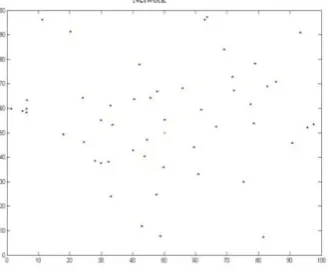
a) Node Deployment

[image:5.595.355.520.582.718.2]

A large number of nodes are deployed in the network. They are deployed in such a way so that they cover the maximum area. Nodes are deployed randomly. They are scattered from environment. No calculation is performed to deploy these sensor nodes.

(6)

b) Function of Pareto Front

The Pareto front shows the output in multi dimensions. Pareto front accepts only those values which lie in its range means if both the factor satisfies the condition. Pareto front accepts only those values in which both the factors perform their own task accurately.

Fig-5: Balancing of Energy and Coverage

From the Fig.-5 it can be seen that there are two factors, energy and coverage. The red colored nodes are covering maximum area and consuming less amount of energy, hence they are satisfying the condition. So, these will be accepted. The blue colored nodes are covering maximum area but consuming a larger amount of energy. Blue nodes are not satisfying the condition. So, these nodes are rejected.

The values of the round number at which the first node, half node and last node dead for the MCSDP(maximum

coverage sensor deployment Problem)[1] and

CEBSP(coverage energy balancing sensor problem)

method is shown in the table.

Table-2: Comparison of dead nodes on the basis of MCSDP [1] and CEBSP method

Comparison MCSDP CEBSP

First node dead 141 150

Half node dead 182 193

Last node dead 306 480

The round number at which the first node dies is known as

First Node dead.

The rounds taken to die the half nodes of the system show the Half Node dead.

The round number at which the last node of the system got dead shows the Last Node dead.

c) FND Comparison

FND stands for First Node dead. The round number at which first node dies is known as First Node dead.

Fig-6: First node comparison

The corresponding graph is shown below which depicts that in the MCSDP[1], at the round number 141 the first node dies whereas, in the CEBSP this round number got increased to 150. Hence, the CEBSP performs better.

d) HND Comparison

HND stands for Half Node dead. Every node has limited energy. If half of nodes from the total deployed nodes go dead, it means half of the nodes of system are dead and the round number at which this occurs is termed as half node dead.

Fig-7: Half node Comparison

(7)

increased to 193.

e) Network Energy Consumption

Remaining energy is the energy which is left after consumption. Our main motive is to maximize the remaining energy. The energy is required to transmit the information to the destination (base station).

Fig-8: Network Energy Comparison

The Energy consumption by nodes should be minimized or the remaining energy should be maximized. For the same number of round, the comparison of MCSDP [1] and CEBSP is performed and CEBSP consumes less amount of energy than MCSDP[1].

f) Last Node Dead Comparison

Fig-9:

Last Node Dead comparison

The round at which the last node of the system got dead is known as Last Node Dead. The Last node dead comparison of MCSDP [1] and CEBSP is shown in the graph which also shows that the CEBSP performs better than the MCSDP

because the last dead node according to CEBSP occurs later than MCSDP [1].

4.3 Summary of Results

In this section, metrices like first node dead, half node dead, last node dead, energy consumption comparison are defined. It is identified that proposed CEBSP performs better than that of MCSDP [1].

5. CONCLUSIONS

In this paper, our main motive is to perform balancing of the energy and coverage means the nodes should be deployed in such a way in which nodes cover the large area and consume less energy and we have achieved that goal (maximizing coverage and minimizing the energy consumption) by applying multi objective genetic algorithm.

REFERENCES

[1]Ozan Zorlu, Ozgur Koray Sahingoz, “Increasing the coverage of Homogeneous WSN by Genetic Algorithm based deployment,” ISBN:978-1-4673-9609-7 2016 IEEE. [2]Shiyuan Jin, Ming Zhou, Annie S. Wu, “Sensor Network

Optimization Using GA,”School of EECS, University of Central Florida Orlando, FL 32816.

[3]NaeimRahmani, FarhadNematy, Amir MasoudRahmani, Mehdi Hosseinzadeh, “Node Placement for Maximum Coverage Based on Voronoi Diagram Using Genetic Algorithm in WSN,” Australian Journal of Basic and Applied Sciences, 5(12): 3221-3232, 2011 ISSN 1991-8178

[4]Yang SUN†, and Jingwen TIAN, “WSN Path Optimization Based on Fusion of Improved Ant Colony Algorithm and

Genetic Algorithm,” Journal of

ComputationalInformationSystems6:5(2010)1591-1599 [5]Seyed Mahdi Jameii and Seyed

MohsenJameii,“Multi-objective Algorithm for Coverage in sensor networks,” IJCSEIT, Vol.3, No.4, August 2013.

[6]S.M. Hosseinirad, and S.K. Basu,“ Wireless sensor network design through genetic algorithm,” Journal of AI and Data Mining Vol. 2, No .1, 2014, 85-96.

[7]Mohammad M. Shurman, Mamoun F. Al-Mistarihi, Amr N. Mohammad, Khalid A. Darabkh, and Ahmad A. Ababnah, “Hierarchical Clustering Using Genetic Algorithm in Wireless Sensor Networks,” MIPRO 2013, May 20-24, 2013, Opatija, Croatia.

[8]Amol P. Bhondekar, RenuVig, C Ghanshyam, MadanLalSingla, and PawanKapur,“GA-BasedNode Placement Methodology for WSN,” IMECS 2009 Vol. 1. [9]Y Yoon and Y H. Kim, "An Efficient Genetic Algorithm

(8)

pp.1473-1483, April 2013.

[10]Y Zou and K. Chakrabarty, "Sensor Deployment and Target Localization Based on Virtual Forces", in Proc. Twenty-Second Annual Joint Conf. of theIEEE Computer and Communications, IEEE Societies, San Francisco, CA, April 2003, pp.1293-1303 vol.2.

[11]C. S. Raghavendra (Editor), Krishna M. Sivalingam (Editor), Taeib F. Znati (Editor). “Wireless Sensor Network”, Springer. 2006.

[12]Shashi Phoha (Editor), Thomas F. La Porta (Editor), Christopher Griffin (Editor). “Sensor Network Operations”,Wiley–IEEE Press. 2006

[13]Adam Dunkels ,Fredrik ¨Osterlind and Zhitao He, “An Adaptive Communication Architecture for Wireless Sensor Networks”, November 6–9, 2007, Sydney, Australia.

[14]Xi CHEN,Qianchuan ZHAO and Xiaohong GUAN, “ENERGY-EFFICIENT SENSING COVERAGE AND

COMMUNICATION FOR WIRELESS SENSOR

NETWORKS”, National Natural Science Foundation (No. 60574087, 60574064) and the “111 International Collaboration Project” of China, feb 2007.

Multi Objective Soft Computing Techniques for Dynamic Deployment in WSN