Enhancement of Power System Performance by Optimal Placement of Distributed Generation using Genetic Algorithms

(1)

Enhancement of Power System Performance by Optimal Placement of

Distributed Generation using Genetic Algorithms

Deependra Kumar Mishra

1

_{, Bindeshwar Singh}

2

1,2_{Kamla Nehru Institute of Technology (KNIT), Sultanpur, Uttar Pradesh, India}

---***---Abstract - In distribution network system, the DGs have many advantages which include decreasing power loss and improvement of voltage profile. These benefits can be achieved if DGs are optimally placed and sized in the system. This paper presents how to improve node voltage, power loss and MVA intake powerin distributed network system due to DGs allocation strategy by using Genetic algorithm (GA). The main contribution of the research work has been to suggest to optimal placement of DGs and use of an optimal power flow based formulation to determine their settings. The suggested methods have been applied on 37-bus distribution systems.

Key Words: Distributed generations (DGs), Distribution networks, Different load models (DLMs), Genetic Algorithm (GA), Power system performances

1. Introduction

DG units are small generating plants connected directly to the distribution network or on the customer site of the meter. In the last decade, the penetration of renewable and non-renewable DG resources is increasing worldwide encouraged by national and international policies aiming to increase the share of renewable energy sources and highly efficient micro-combined heat and power units in order to reduce greenhouse gas emissions and alleviate global warming [1]. Electric utilities are now continuously searching upcoming new technologies to provide acceptable power quality and higher reliability to valuable customers. Non-conventional generation is growing more rapidly around the world due to its low size, low cost and less environmental impact with high potentiality. Investment in DG enhances environmental benefits particularly in combined heat and power applications [2].

1.1Contribution of paper

In this paper, the different type of DGs with DLMs in distribution systems for enhancement of power system performances using GA. The comparisons of results are also presnted in this paper.

1.2 Organization of paper

The organisation of paper are as follws: Section 2 discusses the mathematical problem formulation. Section 3 introduces the GA. Section 4 discusses the simulation results and

discussions. Section 5 introduces the conclusion of this paper and future scope of work.

2. Mathematical Problem Formulation

The mathematical models of DGs are explained in sub-sections 2.1-2.3, respectively [3]-[5].

2.1 General

For different types of load like as constant load models, industrial load models, residential load models, commercial load models, reference load models, the effect of different types of DGs i.e. DG-1, DG-2, DG-3, DG-4 an IEEE-38 bus distribution system is taken for simulation. The DG planning is to reduce the real power loss in distribution network. With some other power system performance indices like as reactive power loss, MVA capacity, voltage profile, and power flow reduction in the distribution network are used as objective function in the form of single or multi objective for optimization [3].

2.1.1 Reduce line loss

The mathematical formulation for loss minimization and objective function (f) is expressed as eq. (1).

_

_ 1

n

i bus i bus

f

P





(1)

_ i bus

P

is the nodal injections of power in a network and n is total number of buses.

2.1.2 Increase capacity of DG

The optimal allocation of DG objective can maximize the DG capacity in eq. (2).

_

_ 1

n

DGi bus i bus

f

P





(2)

_ DGi bus

P

is the DG capacity of

i

_thbus.

2.1.3 Enhance socio-economic culture

(2)

associated with social welfare has been formulated as eq(3)-(4).

_ _ _ _ _

_ 1

(

)

(

)

(

))

n

i bus Di bus i bus Di bus DGi bus

i bus

f

B

P

C

P

C P







(3)

_ _ _ _

Pr

ofit

i bus





i bus



P

DGi bus



C P

(

DGi bus

)

₍₄₎

_ DGi bus

P

is the DG Size at node i,

B P

i

(

Di

)

_{is quadratic}

benefit curve submitted by buyer (DISCO), minus quadratic bid curve submitted by seller (GENCO)

C P

_i

(

_Di

)

, minus the quadratic cost function supplied by DG owner

C P

(

_DGi

)

.



i denotes location margin price and

C P

(

_{DGi bus}_{_}

)

is cost characteristic at node i.

2.1.4 Complex objectives

The complex objective aims are minimize the cost of setting up of DGs, DGs investment, DGs operational cost and total expenses toward compensating for system losses. Objective of this content to reduce the investment and operating costs of DGs, expenses toward purchasing the required extra power by the DISCO.

2.1.5 Load modeling

Planning of DGs for different load Models, a IEEE 38 distribution bus system is adopted. the line impedances, load data and line power limits are expressed in p.u. at the base voltage of 12.66 kV and base MVA of 10 MVA. In conventional load flow analysis the active and reactive power loads are assumed as constant power loads whereas in practice the loads may be voltage dependent. voltage dependent load model is a static load model that represents power relationship to the voltage as exponential equation and represented in eq. (5)-(6).

_{_} _{0 _} _

0 _

alpha i bus i bus i bus

i bus

V

P

V











_

_





(5)

_

_ 0 _

0 _ beta i bus i bus i bus

i bus

V

Q

V



















(6)

Where, Pi_bus, Qi_bus, P0i_bus, Q0i_bus, Vi_bus, and V0i_busare in per unit. Above eq. (5) and (6) neglect the frequency dependence of distribution system load. In practice, the load on each bus may be the composition of constant load models, industrial load models, residential load models, commercial load models, reference load models. the different load models at each bus is considered as described and represented in following form as eq. (7)-(8).

(7)

(8)

Where, alphac and betac are active and reactive exponents for constant load model alphai and betai are active and reactive exponents for industrial load model; alphar and

betar are active and reactive exponents for residential load model; alpham and betam are active and reactive exponents for commercial load model; alphaf and betaf are active and reactive exponents for reference load model. wc_pi_bus, wi_pi_bus,

wr_pi_bus, wm_pi_bus and wf_pi_busare the relevant factors for active constant, industrial, residential, commercial and reference Load models at bus i. wc_qi_bus, wi_qi_bus, wr_qi_bus, wm_qi_bus and

wf_qi_bus are the relevant factors for reactive costant, industrial, residential, commercial and reference Load models at bus i. The following condition must be satisfied for all buses except buses without load (BWL) (Bus 1 is slack bus and buses 34 to 38 are not having load) in equs. (9)-(10).

for i=1 to NB, but i_bus ≠BWL (9)

for i=1 to NB, but i_bus ≠BWL (10)

2.2 DG modeling

The formulation of DGP problem is proposed on the basis of two objective functions such as real power loss and apparent power intake [10].

(i) Minimization of real power loss of the system

(3)

2 2

_ _

2

_ 2 _

, _

_ L

ij bus ij bus

L ij bus ij bus

i j bus N

i bus

P

Q

P

r

V









(11)

The PL is function of all system bus voltage (Vi_bus), line resistances (ri,j_bus), alpha, and beta. The total losses mainly depend on voltage profile.

(ii) Minimization of total MVA intake at main substation

The objective function is apparent power intake (Sint) at main substation. The Pint is the sum of PD and PL, and represented by eq. (12)-(13).

(12) Similarly, the Qintis the sum of QDand QL, and represented by eq. (13).

(13) Apparent power intake at main substation is expressed as equ. (14).

S

int



[(

P

int

)

2



(

Q

int

) ]

2 1/ 2 (14) And apparent power requirement for distribution system is expressed as equ. (15).

2 2 1/2

int int

[(

)

(

) ]

sys DG DG

S



P



P



Q



Q

(15) It is observed that for a distribution system in equs. (16)-(17).

0 _ 0 _

_ 1

(

/

)

B N

alpha i bus i i bus L i bus

P

V

P







(16)

0 _ 0 _

_ 1

(

/

)

B N

beta i bus i i bus L i bus

Q

V

Q







(17) Thus the Pint and Qint in equs. (12)-(13) respectively are largely decided by the load exponents, alpha and beta, not by PLand QL.

V

min



V

i bus_



V

max₍₁₈₎

max

, _ , _

i j bus i j bus

S



CS

₍₁₉₎

P

DG



P

int₍₂₀₎

Where, Vmin= 0.95 p.u., Vmax= 1.03 p.u.,

max , _ i j bus

CS

_{is the}

power capacity limit.

2.3 Power system performance indices [12]-[14]

(i)

Real Power Intake Index (PI_Index)

The real power intake index is defined as:

100 _

_





WODG WDG

Index

PI

Index

PI

Index

PI

(21)

this index indicate reduction in Pint and more capacity release of substation. where, PWODG= 3.9039

(ii)

Reactive Power Loss Index (QI_Index)

The reactive power intake index is defined as:

100 _ _ _   WODG WDG Index QI Index QI Index QI (22)

The lower values of this index indicate reduction in Qint.

where, QWODG= 2.4259

(iii)

Voltage Deviation Index (VD_Index)

The voltage deviation index is defined as:

100 _

_





WODG WDG

Index

VD

Index

VD

Index

VD

(23) It is related to maximum voltage drop between each node and root node. The lower values of this index indicate better performance of the network. where, VREF=1.0300

(iv)

Apparent Power Intake (Sint) Index (SI_Index)

The Apparent Power Intake Index is defined as:

100 _ _ _   WODG WDG Index SI Index SI Index

SI (24)

The lower values of this index indicate reduction in Sint ,and more capacity release of substation. where, SWODG= 4.5962

(v)

Real Power Index (PL_Index)

The real power loss index is defined as: 100 _ _ _   WODG WDG Index PL Index PL Index PL (25) The lower value of this index indicates better benefits in terms of real power loss reduction accrued due to DG location & size. Where, Min. LossWODG = 0.1889

(vi)

Real Power Penetration of DG (DG_P)

The ratio of the amount of DG active power injected into the network to the summation of active power with DG

and without DG.

_



100 



WDG WODG WDG

P

DG

(26)

(vii) Reactive Power Penetration of DG (DG_Q)

The ratio of the amount of DG reactive power injected into the network to the summation of reactive power with DG and without DG.

(4)

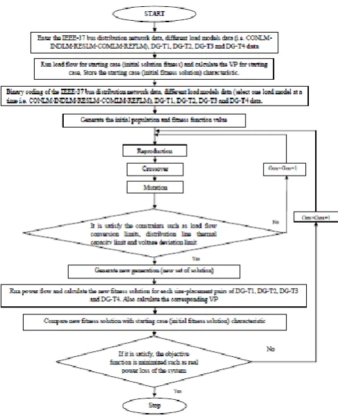
[image:4.595.47.291.230.533.2]

A powerful class of optimization methods is the family of GA. The GA become particularly suitable for the problem posed here. GA based on power loss minimization and energy loss optimization technique is proposed for finding size and site for DG to place in power systems. If network structure is fixed, all branches between nodes are known and evaluation of the objective functions depends only on the size and location of DG units [3].

Fig. 1: The flowchart of GA for optimal placement and sizing of DG in distribution systems

GA that yields good results in many practical problems is composed of three operators:

(i) Crossover: The individuals, randomly organized pair-wise, have their space locations combined, in such a way that each former pair of individuals gives rise to a new pair.

(ii) Mutation: Some individuals are randomly modified, in order to reach other points of the search space.

(iii) Selection: The individuals, after mutation and

crossover, are evaluated. They are chosen or not chosen for being inserted in the new population through a probalistic rule that gives a greater probability of selection to the “better” individuals. The advantages in using GA are that they require no knowledge or gradient information about the response

surface; they are resistant to becoming trapped in local optima and they can be employed for a wide variety of optimization problems.

4. Simulation Results and Discussions

4.1 General

The simulation results and discussions corresponding to DG-T1, DG-T2, DG-T3 and DG-T4 type operating at power factors 1.00, 0.85 leading, 0.00 and 0.85 lagging, respectively.

4.2 IEEE 37 Bus (38 Node) Test System and its Data

The IEEE 37 bus (38 nodes) test system and its data are given in Fig. 4 and Table 1, respectively.

[image:4.595.322.553.309.516.2]

Fig. 2: IEEE 37 bus (38 node) test system [3]

Table 1: Line parameter and load data for 37 buses (38 nodes) test system [3]

F T Line impedance (p. u.) L _(p.uSL )

Load on the bus (p. u.)

R X P Q 1 2 0.0005

74 0.000293 1 4.60 0.10 0.06 2 3 0.0030

70 0.001564 6 4.10 0.09 0.04 3 4 0.0022

79 0.001161 11 2.90 0.12 0.08 4 5 0.0023

73 0.001209 12 2.90 0.06 0.03 5 6 0.0051

00 0.004402 13 2.90 0.06 0.02 6 7 0.0011

(5)

30 4 3 0 0 8 9 0.0064

13 0.004608 25 1.05 0.06 0.02 9 10 0.0065

01 0.004608 27 1.05 0.06 0.02 1

0 11 0.001224 0.000405 28 1.05 0.04 0.03 1

1 12 0.002331 0.000771 29 1.05 0.06 0.03 1

2 13 0.009141 0.007192 31 0.50 0.06 0.03 1

3 14 0.003372 0.004439 32 0.45 0.12 0.08 1

4 15 0.003680 0.003275 33 0.30 0.06 0.01 1

5 16 0.004647 0.003394 34 0.25 0.06 0.02 1

6 17 0.008026 0.010716 35 0.25 0.06 0.02 1

7 18 0.004538 0.003574 36 0.10 0.09 0.04 2 19 0.0010

21 0.000974 2 0.50 0.09 0.04 1

9 20 0.009366 0.008440 3 0.50 0.09 0.04 2

0 21 0.002550 0.002979 4 0.21 0.09 0.04 2

1 22 0.004414 0.005836 5 0.11 0.09 0.04 3 23 0.0028

09 0.001920 7 1.05 0.09 0.05 2

3 24 0.005592 0.004415 8 1.05 0.42 0.20 2

4 25 0.005579 0.004366 9 0.50 0.42 0.20 6 26 0.0012

64 0.000644 14 1.50 0.06 0.02 2

6 27 0.001770 0.000901 15 1.50 0.06 0.02 2

7 28 0.006594 0.005814 16 1.50 0.06 0.02 2

8 29 0.005007 0.004362 17 1.50 0.12 0.07 2

9 30 0.003160 0.001610 18 1.50 0.20 0.60 3

0 31 0.006067 0.005996 19 0.50 0.15 0.07 3

1 32 0.001933 0.002253 20 0.50 0.21 0.10 3

2 33 0.002123 0.003301 21 0.10 0.06 0.04 8 34 0.0124

53 0.012453 24 0.50 0.00 0.00 9 35 0.0124

53 0.012453 26 0.50 0.00 0.00 1

2 36 0.012453 0.012453 30 0.50 0.00 0.00 1

8 37 0.003113 0.003113 37 0.50 0.00 0.00 2

5 38 0.003113 0.002513 10 0.10 0.00 0.00

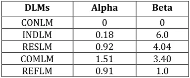
[image:5.595.339.531.157.236.2]

4.3 Real and reactive power exponential indexes for DLMs [9]

Table 2: Exponential indexes of DLMs

DLMs Alpha Beta

CONLM 0 0

INDLM 0.18 6.0

RESLM 0.92 4.04

COMLM 1.51 3.40

REFLM 0.91 1.0

4.4 Comparison of Results with Different type of DGs

[image:5.595.303.564.443.655.2]

The comparison of power system performance parameters such as Real power intake index (PI_Index), Reactive power intake index (QI_Index), Voltage deviation index (VD_Index), Apparent power intake index (SI_Index), Real power loss index (PL_Index), Real power penetration of DG (DG_P), Reactive power penetration of DG (DG_Q) with respect to DLMs such as constant, industrial, residential, commercial and reference load models are for DG-T1 type, DG-T2 type, DG-T3 type and DG-T4 type operating at different power factors such as 1.00, 0.85 leading, 0.00 and 0.85 lagging, respectively are shown in Fig. 3-9.

Table 3: Comparison of simulation results of PI_Index for different types of DGs with DLMs

PI_Index CONLM INDLM RESLM COMLM REFLM DG-T1 47.66 23.88 21.21 40.63 46.32 DG-T2 37.07 17.94 15.57 36.04 35.21 DG-T3 49.51 28.23 25.58 43.21 49.15 DG-T4 48.68 25.33 23.40 41.71 47.64

Fig. 3: PI_Index with DLMs

Table 4: Comparison of simulation results of QI_Index for different types of DGs with DLMs

QI_Ind

ex CONLM INDLM RESLM COMLM REFLM

(6)

[image:6.595.312.558.63.282.2]

DG-T4 47.53 23.18 25.34 39.60 46.52

Fig. 4: QI_Index with DLMs

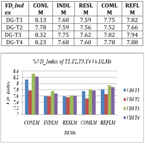
Table 5: Comparison of simulation results of VD_Index for different types of DGs with DLMs

VD_Ind

ex CONLM INDLM RESLM COMLM REFLM DG-T1 8.13 7.60 7.59 7.75 7.82 DG-T2 7.78 7.59 7.56 7.52 7.66 DG-T3 8.32 7.75 7.62 7.82 7.94 DG-T4 8.23 7.68 7.60 7.78 7.88

Fig. 5: VD_Index with DLMs

Table 6: Comparison of simulation results of SI_Index for different types of DGs with DLMs

SI_Inde

[image:6.595.35.286.100.290.2]

x CONLM INDLM RESLM COMLM REFLM DG-T1 40.48 20.28 18.02 36.51 39.69 DG-T2 37.04 17.92 15.48 34.01 35.19 DG-T3 44.49 24.05 23.96 41.97 43.69 DG-T4 42.64 22.22 19.39 39.68 41.61

[image:6.595.311.554.341.589.2]

Fig. 6: SI_Index with DLMs

Table 7: Comparison of simulation results of PL_Index for different types of DGs with DLMs

PL_Index CONL

[image:6.595.42.280.359.601.2]

M INDLM RESLM COMLM REFLM DG-T1 53.66 55.05 62.99 66.34 53.89 DG-T2 43.67 51.03 54.57 65.96 44.20 DG-T3 69.08 69.66 68.34 69.50 68.81 DG-T4 55.97 57.31 63.50 67.64 55.67

Fig. 7: PL_Index with DLMs

Table 8: Comparison of simulation results of DG_P for different types of DGs with DLMs

DG_P CONLM INDL

(7)

[image:7.595.49.279.96.243.2] [image:7.595.40.290.300.514.2]

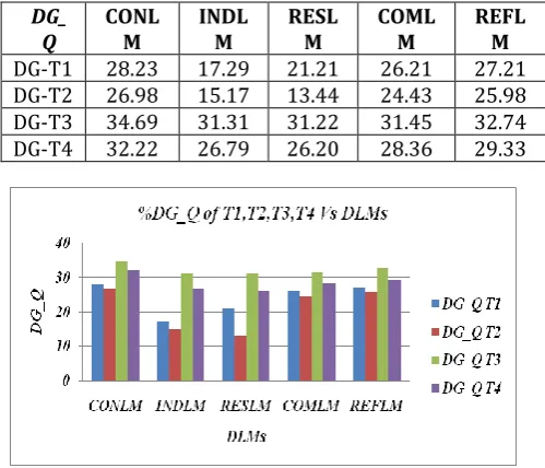
Table 9: Comparison of simulation results of DG_Q for different types of DGs with DLMs

DG_

Q CONLM INDLM RESLM COMLM REFLM DG-T1 28.23 17.29 21.21 26.21 27.21 DG-T2 26.98 15.17 13.44 24.43 25.98 DG-T3 34.69 31.31 31.22 31.45 32.74 DG-T4 32.22 26.79 26.20 28.36 29.33

Fig. 9: DG_Q with DLMs

5. Conclusions

In this work different load model such as constant, industrial, residential, commercial and reference load models, at every bus for different type of DG such as DG-T1, DG-T2, DG-T3, DG-T4 are considered The DG planning based gives appropriate result. It is desirable to keep the DG Planning indices i.e. Real power intake index (PI_Index), Reactive power intake index (QI_Index), Voltage deviation index (VD_Index), Apparent power intake index (SI_Index), Real power loss index (PL_Index), Real Power Penetration of DG (DG_P), Reactive Power Penetration of DG (DG_Q) below the limits which are defined without DG conditions. Proper sizing and location of DG can reduce losses, reduce MVA intake power, improve voltage profile, increase the loadability of system and reduce the real and reactive power losses of the system. DG-T2 type shows the best result in all the types of DGs. DGs performance order of DG-T2 > DG-T1 > DG-T4 > DG-T3.

REFERENCES

[1] Pavlos S. Georgilakis, Optimal Distributed Generation

Placement in Power Distribution Networks: Models, Methods, and Future Research. IEEE Transactions on Power Systems 2013; 28(3): 3420-3428.

[2] S. K. Saha, S . Banerjee, D. Maity and C. K. Chanda,

Optimal Sizing and Location Determination of Distributed Generation in Distribution Networks. IEEE Transactions on Power Systems 2015; 1-5.

[3] Deependra Singh, Devender Singh, and K. S. Verma, GA

based Optimal Sizing & Placement of Distributed Generation for Loss Minimization. International Journal of Electrical, Computer, Energetic, Electronic and Communication Engineering 2007; 1(11): 1604-1610.

[4] Bindeshwar Singh, K.S. Verma, Deependra Singh and

S.N. Singh, A novel approach for optimal placement of distributed generation & facts controllers in power systems: an overview and key issues. International Journal of Reviews in Computing 2017; 7: 29-54.

[5] Duong Quoc Hung, Nadarajah Mithulananthan and R. C.

Bansal, Analytical Expressions for DG Allocation in Primary Distribution Networks. IEEE Trans. On Energy Conversion 2010; 25(3): 814-820.

[6] Devender Singh, R. K. Mishra, and Deependra Singh, Effect of Load Models in Distributed Generation Planning. IEEE Trans. On Power Systems 2007; 22(4): 2204-2212.

[7] Thomas Ackermann, Go ran Andersson and Lennart So

der, Distributed generation: a definition. Electric Power Systems Research 2001; 57: 195–204.

[8] Rajendra Prasad Payasi, Asheesh K. Singh and

Devender Singh, Review of distributed generation planning: objectives, constraints, and algorithms. International Journal of Engineering, Science and Technology 2011; 3(3): 133-153.

[9] IEEE Task Force on Load Representation for Dynamic Performance, Standard Load Models for Power Flow and Dynamic Performance Simulation. IEEE Trans. on Power Systems. 1995; 10(3): 1302-1313.

[10], K.S. Verma, Deependra Singh and S.N. Singh, A Novel

Approach for Optimal Placement of Distributed Generation & FACTS Controllers in Power Systems: An Overview and Key Issues. International Journal of Reviews in Computing 2011; 7: 29-54.

[11]R.K. Singh and S.K. Goswami, Optimum allocation of

distributed generations based on nodal pricing for profit, loss reduction, and voltage improvement including voltage rise issue. Electrical Power and Energy Systems 2010; 32: 637–644.

[12]Rajendra P. Payasi, Asheesh. K. Singh and Devender

(8)

[13]Deependra Singh, Devender Singh and K. S. Verma,

Multi-objective Optimization for DG Planning With Load Models. IEEE Transactions on Power Systems 2009; 24(1): 427-436.

[14]Rajendra Prasad Payasi, Asheesh K. Singh and

Devender Singh, Planning of different types of distributed generation with seasonal mixed load models. International Journal of Engineering, Science and Technology 2012; 4(1): 112-124.

[15]IEEE Task Force on Load Representation for Dynamic

Performance, Load representation for dynamic performance analysis. IEEE Trans. Power System 1993; 8(2): 472-482.

BIOGRAPHIES

Deependra Kumar Mishra received the B.Tech. degree in electrical and electronics engineering from BBSCET, Allahabad (U.P.), in 2010 from GBTU, Lucknow, India and pursuing the M.Tech.(PT) degree in power system (electrical engineering) from Kamla Nehru Institute of Technology, Sultanpur (U.P.) from AKTU, Lucknow, India. His research interests are distributed generation planning and distribution system analysis. he is an Assistant Professor with Department of Electrical and electronics Engineering, BBSCET, Allahabad, U.P., India.