A two level domain decomposition algorithm for linear complementarity problem

R E S E A R C H

Open Access

A two-level domain decomposition algorithm

for linear complementarity problem

Shuilian Xie

_{, Zhe Sun}

_{and Yuping Zeng}

*_{Correspondence:}

[email protected] 1_{School of Mathematics, Jiaying}

Univiersity, Meizhou, Guangdong 514015, P.R. China

Full list of author information is available at the end of the article

Abstract

In this paper, a two-level domain decomposition algorithm for linear

complementarity problem (LCP) is introduced. Inner and outer approximation sequences to the solution of LCP are generated by the proposed algorithm. The algorithm is proved to be convergent and can reach the solution of the problem within finite steps. Some simple numerical results are presented to show the effectiveness of the proposed algorithm.

1 Introduction

In this paper, we consider the following linear complementarity problem (LCP) of finding

u∈Rn_{such that}

u≥, F(u)≥, uTF(u) = , (.)

whereF(u) =Au+b,Ais anM-matrix,b∈Rn_{is a given vector.}

LCP is a wide class of problems and has many applications in such fields as physics, optimum control, economics,etc.As a result of their broad applications, the literature in this field has benefited from contributions made by mathematicians, computer scientists, engineers of many kinds, and economists of diverse expertise. There are many surveys and special volumes (see,e.g., [–] and the references therein).

Domain decomposition techniques are widely used to solve PDEs since ’s. This kind of techniques attracts much attention, since it is portable and easy to be parallelized on parallel machines. It has been applied to solve various linear and nonlinear variational inequality problems, and the numerical results show that it is efficient, see, for example, [–]. It contains many algorithms, such as classical additive Schwarz method (AS), mul-tiplicative Schwarz method (MS), restricted additive Schwarz method (RAS), and so on. In [], a variant of Schwarz algorithm, called two-level additive Schwarz algorithm (TLAS), was proposed for the solution of a kind of linear obstacle problem. This method can divide the original problem into subproblems in an ‘efficient’ way. In other words, the domain is decomposed in different way at each step and the dimensions of the subproblems we deal with are lower than that of the original problem. The numerical results show that the TLAS is significant. In [], the TLAS is extended for the nonlinear complementarity problem with anM-function. The algorithm offers a possibility of making use of fast non-linear solvers to the subproblems, and the choice of the initial is much easier than that of the TLAS. Another efficient way to solve problem (.) is given by semismooth Newton

methods (e.g., see [, ]). This method is attractive, because it converges rapidly from any sufficiently good initial iterate, and the subproblems are also systems of equation. An active set strategy is also an efficient way to solve discrete obstacle problems, see, for ex-ample, [–]. Based on some kind of active set strategy, the discrete obstacle problem can be reduced to a sequence of linear problems, which are then solved by some efficient methods. In this paper, we combine the idea of the active set strategy with the thought of TLAS,i.e., constructing inner and outer approximation sequences to the solution of LCP, and present a two-level domain decomposition algorithm. As we will see in the sequel, the main difference between the two-level domain decomposition algorithm (TLDD) and TLAS discussed in [] lies in the way of constructing the outer approximation of the solu-tion. What’s more, with the idea of an active set strategy, the TLDD may be easier extended to other problems, such as bilateral obstacle problem.

The paper in the sequel is organized as follows. In Section , we give some preliminaries and present a two-level domain decomposition algorithm for problem (.). In Section , we discuss the convergence of the algorithm proposed in Section . In Section , we report some simple numerical results.

2 Preliminaries and two-level domain decomposition algorithm

In this section, we give some preliminaries and present a two-level domain decomposition algorithm for solving problem (.).

Firstly, similarly to [, ], we introduce two operators, which will be useful in the con-struction of the algorithm in this paper. LetN={, , . . . ,n}. LetI,Jbe a nonoverlapping decomposition ofN. That is,N=I∪JandI∩J=∅. For anyv∈Rn, we introduce the following linear problem of findingw∈Rn_{such that}

wI=vI, FJ(w) = , (.)

wherevIdenotes the subvector ofvwith elementsvj(j∈I). Similar notation will be used

in the sequel. We denote linear system (.) above by the operation form

w=GJ(v).

Similarly, we introduce the following problem of findingw∈Rn_{such that}

wI=vI, min

FJ(w),wJ

= . (.)

We denote nonlinear problem (.) above by the operation form

w=TJ(v).

Theorem .[] Problem(.)is equivalent to the following variational inequality of find-ing u∈Rn_{such that}

Theorem .[] The solution of problem(.),or equivalently(.),is unique and is the minimal element of S,where S is the supersolution set of problem(.),which is defined by

S=v∈Rn:v≥and F(v)≥.

Similarly, we have the following theorem.

Theorem . The solution of problem(.),or equivalently(.),is unique and is the max-imal element of U,where U is the subsolution set of problem(.),which is defined by

U=v∈Rn:v≥andminv,F(v)≤.

Based on Theorems . and ., we can construct the following additive Schwarz algo-rithm for LCP (.).

Algorithm .(Additive Schwarz algorithm with two subdomains) LetIandJbe a de-composition ofN,i.e.,I∪J=N. Givenu_{∈S. Fork= , , . . . , do the following two steps}

until convergence.

Step : Solve the following two subproblems in parallel

⎧ ⎨ ⎩

finduk,_∈Kk,_{such that}

(FI(uk,),vI–uIk,)≥, ∀v∈Kk,,

⎧ ⎨ ⎩

finduk,_∈Kk,_{such that}

(FJ(uk,),vJ–uJk,)≥, ∀v∈Kk,,

where

Kk,=v∈Rn:v–uk_N\I= ,

Kk,=v∈Rn:v–uk_N\J= .

Here we defineN\I={j∈N:j∈/I}for any subsetIofN.

Step :uk+=min(uk,,uk,), where ‘min’ should be understood by componentwise. Similar to the proof of Theorem . in [], we have the following convergence theorem for Algorithm ..

Theorem . Let the sequence{uk_{}be generated by Algorithm..For k= , , . . . ,we have}

(a) uk,i≤uk,i= , and thenuk+≤uk, (b) uk,i_{∈S,i= , and thenu}k+_∈S,

(c) lim_k→∞uk_=u,

where u is the solution of problem(.).

In what follows, we letN_={j∈N:u

j= },N+={j∈N:uj> }, whereuis the

inSand monotonically decreases and converges to the solution. Hence, if we define the coincidence set ofuk_{as follows}

Ik=j∈N:uk_j = , (.)

we have by the monotonicity of{uk}such that

Ik⊆Ik+⊆N, k= , , . . . .

Actually, this gives inner approximations for the coincidence setN_.

There are many algorithms based on active set strategy. Based on some kind of criterion, the index set is divided into two parts: active set and inactive set. We only need to calculate the simplified linear system related to the inactive set. We also draw on the experience of active set strategy to derive the outer approximations for the coincidence set. To be precise, we define

Ok=j∈N:wk_j =  andFj

wk≥, Lk=N\Ok, k= , , . . . , (.) and defineCk_as

Ck=N\Ik∪Lk. (.)

Ckmay contain both elements ofNandN+. So, it is called the critical subsets. Let

ˆ

Ck=Ck∪Hk, (.)

whereHk_{is a subset ofNcorresponding to an overlapping of the subsets associated with}

Lk_andCk_{. That isH}k_⊂Lk_andHk_=Cˆk_∩Lk_.

Now, we are ready to present two-level domain decomposition algorithm for prob-lem (.).

Algorithm .(Two-level domain decomposition algorithm) . Initialization.k:= :

(a) Choose an initialu_{,wsuch thatu}_{∈Sandw∈U. Define the coincidence setI}

according to (.). (b) Solvew_{such that}

⎧ ⎨ ⎩

w_i = , i∈Iorwi= ,Fi(w)≥,

Fi(w) = , otherwise,

(.)

and defineL_,C_andCˆ_{according to (.), (.) and (.), respectively.}

. Iteration step:

(a) Inner approximation (additive Schwarz algorithm with two subdomains). Solve the following two subproblems in parallel:

(i) The subproblem defined by the following obstacle problem

uk,=TCˆk

(ii) The subproblem defined by the following linear equation

uk,=G_Lk

uk. (.)

Letuk+=min(uk,,uk,)and define the coincidence setIk+according to (.). (b) Outer approximation. Solve the linear system

⎧ ⎨ ⎩

wk+

i = , i∈Ik+orwik= ,Fi(wk)≥,

Fi(wk+) = , otherwise.

(.)

IfF(wk+_{)≥, then stop;w}k+_{is the solution. Otherwise, defineL}k+_andCˆk+_according

to (.) and (.), respectively, and letk:=k+  and return to step .

Remark . The subproblems in PSOR method and classical Schwarz algorithm are ob-stacle problems, while the subproblems (.) and (.) can be solved by the use of fast linear solvers.

Remark . The difference between Algorithm . and Algorithm . in [] lies on the way of generating the outer approximation sequence. Algorithm . in [] seems difficult to extend to other problems, such as bilateral obstacle problem, while the idea of Algo-rithm . may be easier to be applied to other problems.

3 The convergence of Algorithm 2.2

In this section, we analyze the convergence of Algorithm .. First, we introduce some lemmas.

Lemma . Let u_{∈S,w∈U and w}_{be defined by(.).Then,we have≤w≤w}_and

w_∈U.

Proof LetIˆ=ˆI∪ ˆI, whereIˆ={i|i∈I},ˆI={i|wi=  andFi(w)≥}andJˆ=N\ ˆI. By

the definition ofw, we havew_ˆ

I=wˆI= . By Theorems . and ., we haveu≥w≥. Hence ifi∈ ˆI, we havewi= . Thenw_Iˆ =wIˆ= . Sincew∈U, we haveFˆJ(w)≤FˆJ(w) = .

Hence, noting thatF(u) =Au+b, andAis anM-matrix, we have ≤w≤w. This

com-pletes the proof.

Lemma . Let u_{∈S,let subsets L}_andCˆ_{be defined by(.)and(.),respectively,}

then

u,=TCˆk

u∈S, u,≤u, (.)

u,=GLu∈S, u,≤u, (.)

u=minu,,u,∈S, (.)

u≤u≤u. (.)

Proof Equation (.) can be directly obtained by Theorem .. By (.), we have

FL

Sinceu_{∈S, we have}

F_L

u≥.

Noticing thatF(u) =Au+b, andAis anM-matrix, (.) concludes

u,≤u. (.)

We have by (.), (.) that

FN\L

u,≥FN\L

u≥. (.)

LetL_=L

 ∪L, whereL ={i∈L|wi = ,Fi(w) < }, andL={i∈L|wi > }. Since

w_∈U,w_{≤u, we haveu}

i>  fori∈L, and thenFL_(u) = . Fori∈L, we havei∈I,

and thenui= . It follows then from (.) andu∈Sthat

u,

N\L_ ≥uN\L, FL

u,=F_L

(u) = , (.)

which meansu,≥u≥. This, together with (.) and (.), implies thatu,∈S. There-fore, (.) holds. Similar to the proof in Theorem ., we have (.) and (.). The proof

is then completed.

By Lemmas . and ., and the principle of induction, we havewk+_≥wk_≥,uk_≥

uk+_{≥,k= , , . . . .}

Lemma . Ok+_⊆Ok_{and I}k_⊆Ik+_⊆N_{,k= , , . . . .If F(w}k+_)≥,wk+_{is the solution.}

Proof Ifj∈Ok+, by the definition ofOk+, we havew_jk+= ,Fj(wk+)≥. Noting that

wk+_≥wk _{≥, we have w}k

j = . IfFj(wk) < , notice that A is an M-matrix, we have

Fj(wk+)≤Fj(wk) < , which is a contradiction. Hence,j∈OkandOk+⊆Ok.Ik⊆Ik+⊆

N_{,k= , , . . . is obvious. Noting (.), it is obvious that if for someksuch thatF(w}k_)≥,

wk_{is the solution.}

Theorem . The sequence generated by two-level domain decomposition method(

Algo-rithm.)converges to the solution u of problem(.)after a finite number of iterations.

Proof If for somek,F(wk_{)≥, by Lemma .,w}k _{is the solution and w}k _{=u since the}

problem (.) has only one solution. Otherwise, sinceuk+_=min(uk,_,uk,_{), we haveI}k,_⊆

Ik+ _{and henceI}k+_\Ik_{= ∅. Noting thatI}k_⊆Ik+ _{and thatN is an index set with finite}

elements,Ik+_\Ik_{=∅can only occur in finite steps. By Lemma ., we haveO}k+_⊆Ok_,

andOk\Ok+=∅also can only occur in finite steps. In this case, after some finite steps, we haveIk+=Ik,Ok+=Ok. By the definition ofwk+, we haveFi(wk+)≥,∀i∈N. Hence, by

4 Numerical experiment

In this section, we present numerical experiments in order to investigate the efficiency of Algorithm .. The programs are coded in Visual C++ . and run on a computer with . GHz CPU. In the tests, we consider the following LCP:

u≥, A(u) –b≥, uTA(u) –b= , (.)

where

A= 

h ⎛ ⎜ ⎜ ⎜ ⎜ ⎜ ⎝

H –I

–I H . ..

. .. ... –I

–I H

⎞ ⎟ ⎟ ⎟ ⎟ ⎟ ⎠ and H= ⎛ ⎜ ⎜ ⎜ ⎜ ⎜ ⎝  – –  . .. . .. ... – –  ⎞ ⎟ ⎟ ⎟ ⎟ ⎟ ⎠ ,

h=√

n+,b= (b,b, . . . ,bn)

T_{is a given vector. In our test, we setb}

i= –.,i= , , . . . ,n/

andbi= .,i=n/ + ,n/ + , . . . ,n.

The matrixAmay be obtained by discretizing the operator –uby using five-point dif-ference scheme with a constant mesh step sizeh= /(m+ ), wheremdenotes the number of mesh nodes inx- ory-direction (n=m_{is the total number of unknowns).}

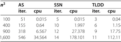
We compare different algorithms from the point of view of iteration numbers and CPU times. Here, we consider three algorithms: classical additive Schwarz algorithm (i.e., Al-gorithm ., denoted by AS), Newton’s method proposed in [] (denoted by SSN), and Algorithm . (denoted by TLDD). In the AS, we decomposeNinto two equal parts with the overlapping sizeO(_). In the algorithms we considered, all subproblems relating to obstacle problems are solved by PSOR with the same relaxation parameterω= ., and the initial point isu=A–ewithe= (, , . . . , )T. The tolerance in the subproblems of the algorithms is chosen to be equal to – _{in ·}

-norm, while in the outer iterative

pro-cesses, it is chosen to be equal to –_{in ·}

-norm. In the TLDD, we choose initialw= .

The tolerance in the subproblems of the algorithms is chosen to be equal to –_{in ·} 

-norm, while in the outer iterative processes, it is chosen to be equal to –in · -norm.

In the SSN, we choose= –_{,p= ,ρ= .,β= ., which is defined by the procedure}

proposed in ([], Section ). We choose the initial pointu_{= .}

Table 1 Comparisons of iteration numbers and cpu times

n AS SSN TLDD iter. cpu iter. cpu iter. cpu

100 51 0.015 5 0.015 3 0.047

400 155 0.64 10 1.997 6 1.154

900 318 6.567 12 27.378 9 17.755

1,600 546 34.564 14 178.101 11 112.117

solve the related linear equations at each iteration step. This may explain why these two algorithms did not perform as well as we expected.

Concluding remark In this paper, we propose a new kind of domain decomposition method for linear complementarity problem and establish its convergence. From the nu-merical result, we can see that this method needs less iteration number to converge to the solution rapidly than the additive Schwarz method and SSN. There are still some in-teresting future works that need to be done. For example, as we can see from TLDD, the main work is calculating the linear equations; we can discuss the affect of inexact solution for related linear subproblems. It is also interesting for us to extend the new method to some other problems, such as nonlinear complementarity problem and bilateral obstacle problem. We leave it as a possible future research topic.

Competing interests

The authors declare that they have no competing interests.

Authors’ contributions

All authors jointly worked on the results and they read and approved the final manuscript.

Author details

1_{School of Mathematics, Jiaying Univiersity, Meizhou, Guangdong 514015, P.R. China.}2_{College of Mathematics and}

Information Science, Jiangxi Normal University, Nanchang, Jiangxi 330022, P.R. China.

Acknowledgements

The work was supported by the Natural Science Foundation of Guangdong Province, China (Grant No. S2012040007993) and the Educational Commission of Guangdong Province, China (Grant No. 2012LYM_0122), NSF (Grand No. 11126147) and NSF (Grand No. 11201197).

Received: 14 June 2013 Accepted: 24 July 2013 Published: 8 August 2013 References

1. Harker, PT, Pang, JS: Finite-dimensional variational inequality and nonlinear complementarity problems: a survey of theory, algorithms and applications. Math. Program.48, 161-220 (1990)

2. Billups, SC, Murty, KG: Complementarity problems. J. Comput. Appl. Math.124, 303-318 (2000)

3. Ferris, MC, Mangasarian, OL, Pang, JS (eds.): Complementarity: Applications, Algorithms and Extensions. Kluwer Academic, Dordrecht (2001)

4. Badea, L, Wang, JP: An additive Schwarz method for variational inequalities. Math. Comput.69, 1341-1354 (1999) 5. Zeng, JP, Zhou, SZ: On monotone and geometric convergence of Schwarz methods for two-sided obstacle problems.

SIAM J. Numer. Anal.35, 600-616 (1998)

6. Jiang, YJ, Zeng, JP: Additive Schwarz algorithm for the nonlinear complementarity problem withM-function. Appl. Math. Comput.190, 1007-1019 (2007)

7. Tarvainen, P: Two-level Schwarz method for unilateral variational inequalities. IMA J. Numer. Anal.19, 273-290 (1999) 8. Xu, HR, Zeng, JP, Sun, Z: Two-level additive Schwarz algorithms for nonlinear complementarity problem with an

M-funcion. Numer. Linear Algebra Appl.17, 599-613 (2010)

9. Luca, TD, Facchinei, F, Kanzow, C: A theoretical and numerical comparison of some semismooth algorithms for complementarity problems. Comput. Optim. Appl.16, 173-205 (2000)

10. Li, DH, Li, Q, Xu, HR: An almost smooth equation reformulation to the nonlinear complementarity problem and Newton’s method. Optim. Methods Softw.27, 969-981 (2012)

11. Hintermüller, M, Ito, K, Kunisch, K: The primal-dual active set strategy as a semismooth Newton method. SIAM J. Optim.13, 865-888 (2002)

13. Kärkkäinen, T, Kunisch, K, Tarvainen, P: Augmented Lagrangian active set methods for obstacle problems. J. Optim. Theory Appl.119, 499-533 (2003)

doi:10.1186/1029-242X-2013-373

Cite this article as:Xie et al.:A two-level domain decomposition algorithm for linear complementarity problem.