Munich Personal RePEc Archive
A New Paradigm: A Joint Test of
Structural and Correlation Parameters in
Instrumental Variables Regression When
Perfect Exogeneity is Violated
Caner, Mehmet and Sandler Morrill, Melinda
North Carolina State University
6 October 2009
Online at
https://mpra.ub.uni-muenchen.de/17689/
A New Paradigm: A Joint Test of Structural and
Correlation Parameters in Instrumental Variables
Regression When Perfect Exogeneity is Violated
Mehmet Caner and Melinda Sandler Morrill
∗October 6, 2009
Abstract
Currently, the commonly employed instrumental variables strategy relies on the knife-edge assumption of perfect exogeneity for valid inference. To make reliable inferences on the structural parameters under violations of exogeneity one must know the true correlation between the structural error and the instruments. The main innovation in this paper is to identify an appropriate test in this context: a joint null hypothesis of the structural parameters with the correlation between the instruments and the structural error term. We introduce a new endogeneity accounted test by combining the structural parameter inference while correcting the bias associated with non-exogeneity of the instrument. To address inference under violations of exogeneity, significant contributions have been made in the recent literature by assuming some degree of non-exogeneity. A key advantage of our approach over that of the previous literature is that we do not need to make any assumptions about the degree of violation of exogeneity either as possible values or prior distributions. In particular, our method is not a form of sensitivity analysis. Since our test statistic is continuous and monotonic in correlation, one can conduct inference for the structural parameters by a simple grid search over correlation values. We can make accurate inferences on the structural parameters because of a feature of the grid search over correlation values. One can also build joint confidence intervals for the structural parameters and the correlation parameter by inverting the test statistic. In the inversion, the null values of these parameters are used. We also propose a new way of testing exclusion restrictions, even in the just identified case.
1
Introduction
Economists frequently apply instrumental variable methods to draw inferences about whether or not a variable influences an economic outcome. For example, labor economists employ varied ∗Caner: North Carolina State University, Department of Economics, 4168 Nelson Hall, Raleigh, NC 27518
instruments, including quarter and year of birth (Angrist and Krueger, 1991), tuition and dis-tance to nearest college (Kane and Rouse, 1995, Card, 1993), attending reform school (Meghir and Palene, 2005) and birth year interacted with school buildings in region of birth (Dufflo, 2001) to measure the extent to which a person’s education influences her salary and wages. In a distinct but related literature that combines macro-economics, political economy and compar-ative institutions, economists employ instruments including early settler mortality (Acemoglu, Johnson and Robinson, 2001), ethnic capital (Hall and Jones, 1999), ethno-linguistic fraction-alization (Mauro, 1995) and legal families (Djankov et al., 2003, and Acemoglu and Johnson, 2006) to determine whether or not the quality of institutions influences long term growth and investment.
Instrumental variable (IV) methods are used to identify causal relationships by isolating changes in an endogenous variable (or variables) that are unrelated to potential unobserved factors. To identify a causal relationship, instruments must be exogenous; that is, they are not related to the outcome variable after controlling for relevant explanatory variables. For example, early settler mortality is exogenous if it is only related to long term growth through its impact on institutions, after controlling for relevant variables such as latitude. This requirement is strong because it means that settler mortality can only influence long term growth indirectly through the quality of contemporary institutions. The exogeneity of early settler mortality, however, is controversial; for example, as noted by Glaeser et al. (2004), early settler mortality could also influence long term growth through its impact on the unobservable human capital of the early settlers. Whether or not the exclusion restriction is perfectly satisfied is debatable for many (and perhaps most) applications of instrumental variables.
Applied econometricians use a simple t-ratio test statistic to infer whether there is causality among the variables analyzed using IV methods. However, the t-test gives unreliable results even when there is a slight violation of exogeneity, as established recently in a paper by Berkowitz, Caner and Fang (2008). As shown in Table 1, the standard t-ratio has undesirable properties when the instrument is endogenous. The table shows the actual size of the test when the single instrument is endogenous. Larger sample sizes exacerbate the problem. For example, with the true correlation of 0.1 at a sample size of n = 100 the size of the test is 19.9%, while if the sample size increases to n = 1000, the size is 88.8%. This is a massive size distortion.
appropriate test is actually a joint test of the structural parameters with the correlation between the structural error and the instruments. Since inferences on the structural parameters depend on this correlation, a joint null is needed. The idea of the test is to subtract the drift from the standard t statistic. The drift depends on the value of the true correlation between the structural error and the instrument. Since the true correlation is between -1 and 1 we can do a grid search over all possible values of the correlation.
In one sense, we propose a test that combines structural parameter inference with a test of violations of exogeneity. The test statistic here is useful for the just identified case as well as the over-identified case. Furthermore, our test can be inverted to get valid confidence intervals for the structural parameters (β0) and the correlation parameter (ρ0) by doing a joint grid search.
We record the values of the test where the null is not rejected as being in the joint confidence interval. We should remind readers that we are not conditioning on one parameter to get the other’s confidence interval. The joint confidence interval can be unbounded with positive probability, so this is a valid confidence interval. The test statistic we derive has standard normal distribution when we have only one endogenous regressor. It has χ2
limit when the number of endogenous regressors are larger than one. So the test is asymptotically pivotal regardless of exogeneity violations. In our most general case, the test statistic takes the minimal value of zero when evaluated at the two-stage least squares estimate of the structural parameter and zero for the correlation parameter. Therefore, the confidence intervals are never empty and contain the two-stage least squares estimate and the zero correlation parameter at every significance level.
One of the key issues is the joint nature of the test. One may be concerned that this would impede inference on the structural parameters alone. In other words, the concern is that one could reject the true null due to usage of the wrong correlation values. In fact, this is not a problem in our context. Since the test statistic is continuous and monotonic in correlation, we will eventually find the true correlation and can conduct inference at that point. If the joint null is true, then the test statistic value will be below the critical values at the true correlation. In that case we do not reject the null and have correct inference. If the alternative is true, our test rejects the false null regardless of correlation values, as does the standard t-test. Therefore even though the joint null may seem to be limiting in interpreting rejection, we can still make accurate inferences on the structural parameters.
no correlation and the structural parameters taking certain values. By testing several possible grid values of the structural parameter, we have several test statistics recorded. If every test rejects the null of no correlation with the structural parameter null value that is tested, then the instrument cannot be exogenous. Simulations show that this has good finite sample properties and can be used in the applied work.
We present two empirical examples that demonstrate the methods we propose. In the first, Acemoglu and Johnson (2005) measure the effects of institutions on country-level gross do-mestic product (GDP) using settler mortality levels as an instrument for the development of institutions. The exclusion restriction requires that early settler mortality rates only affect GDP through the development of institutions. According to the empirical exercise described in Section 5, we find a region of non-rejection that is clearly bounded away from the structural parameter equaling zero. This is a very powerful result because it demonstrates that we can still infer that the coefficient on institutions is positive and statistically significant. Since a perfectly exogenous instrument is very difficult (or perhaps impossible) to find, our test allows researchers to understand the regions where the joint null fails to reject, yielding a joint confidence interval for the correlation and structural parameters.
In addition to the Acemoglu and Johnson example, we demonstrate this method using an example from labor economics. In Card (1995), the author argues that proximity to college can be used as an instrument for college attendance when calculating the returns to schooling on wages. One potential violation of exogeneity is that proximity to college is correlated with other unobserved factors that are positively associated with high earnings, such as having well-educated parents or having a higher quality public primary and secondary education. Although the original estimates indicated statistical significance, we demonstrate that in this case the confidence interval for the structural parameter is unbounded in both directions. Section 5 includes a detailed discussion of the interpretation and implication of these results.
samples, the block size choice is important in their resampling scheme.
Other related and important papers include Nevo and Rosen (2009), where they provide analytical bounds on structural parameters via set identification. Ashley (2009) provides a sensitivity analysis for the instrumental variable regression based on the covariance between the instruments and the structural error. That study shows clearly that correlation plays an important role in inference for structural parameters. He modifies the structural equation so that the new error is orthogonal to the existing instrument. Then he derives the limit for this new two stage least squares estimator. A very recent paper by Guggenberger (2009) considers the several variants of subsampling to gather information about local violation of exogeneity in identification robust tests. He shows that even though the Anderson-Rubin test is oversized, compared to other identification robust test the Anderson-Rubin test performs well. Caner (2009) also considers a similar problem, and shows that Anderson-Rubin test is robust to local violations of exogeneity in the many moments framework. In this paper we do not analyze the Anderson-Rubin test. Rather, we focus on the standard t-test, upon which almost all of the applied literature relies. In the future, we plan to extend our analysis to incorporate modifications to the Anderson-Rubin test.
For Bayesian analysis on the issue of violations of exogeneity in instrumental variables, two good sources are by Conley, Hansen, Rossi (2007) and Kray (2008). Conley, Hansen, and Rossi (2007) consider a three way attack on the problem of violation of exogeneity. The first attempt is to assume a support for the parameter that controls the violation and then use that assumption to build confidence intervals for the structural parameters. This proves to be conservative. The second approach they take is to put a prior on the parameter for the violation and then build confidence intervals for the structural parameters. The third line of attack is fully Bayesian and puts a prior on parameter controlling the violation of exogeneity but allows this parameter to be independent from the structural parameters priors. Then a variant of that is to assume the priors are dependent on each other.
cor-relation parameter. This changes the paradigm of inference in instrumental variable regression and provides a framework that is tractable and straightforward to implement empirically.
The remaining sections of this paper are as follows. Section 2 provides a theoretical basis for the empirical technique. In Section 3, we present an algorithm that suggests a new exogeneity accounted test that reflects the joint nature of the null hypothesis. Section 4 presents simulation results which justify the practicality and efficiency of our estimates. Section 5 presents the two examples of the application of this technique in empirical research. Section 6 provides a discussion and concludes. The proofs are included in Appendix A, and the Stata code used to implement the test statistic is included in Appendix B.
2
The Model and Assumptions
We consider the following linear simultaneous equations model:
y=Xβ0+u, (1)
X =Zπ0+V, (2)
where we refer to (1) as the structural equation and (2) as the first stage equation. Here, X
represents n×k matrix, Xi is a k ×1 vector of endogenous variables, and Z is n×l matrix. Below, Zi is l ×1 vector of instruments, l ≥ k. Also π0 is of full column rank k. The errors ui, Vij, i = 1,· · ·, n, j = 1,· · ·, k are correlated. Control variables may be added to the system. If this is the case, one can simply project them out and the analysis below follows. The variance matrix EViV′
i = ΣV V < ∞, and nonsingular. Eu2i = σ 2
u < ∞, and Eui = EVi = 0. Let ˆβ
represent the two-stage least squares (2SLS) estimate of β0, and ˆπ is the least squares (LS)
estimate of π0.
Assumption 1. (i). (Violation of Exogeneity)
EZiui =C,
where C is l ×1 vector with C = (C1,· · ·, Cm,· · ·, Cl)′, and each Cm 6= 0 and is finite for m = 1,2,· · ·, l.
(ii). We also have
(iii). EZiX′
i has full column rank.
Assumption 2. The following limits hold jointly when the sample size n converges to infinity:
(i).
n−1 n X
i=1 u2
i, n− 1
n X
i=1
Viui, n−1 n X i=1 ViV′ i ! p
→(σ2
u,ΣV u,ΣV V),
where σ2
u,ΣV u,ΣV V are scalar, k×1, andk×k, respectively. The scalar is positive, the vector
is nonzero and finite, and the matrix is positive definite and finite. (ii). We have the following law of large numbers
ˆ
Qzz =n−1 n X
i=1 ZiZ′
i p
→Qzz,
where Qzz is a positive definite and finite k×k matrix. (iii). We have the following central limit theorem
n−1/2 n X
i=1
(Ziui−EZiui), n− 1/2
n X
i=1 ZiVi′
! d
→(Ψzu,ΨZV),
ΨZu
ΨZV
≡N[0,Σ⊗Qzz],
and Σ = σ 2
u Σ′V u
ΣV u ΣV V .
Note that Assumption 1i is the main issue of this paper. The perfect exogeneity that is used instrumental variable analysis is a knife-edge, unrealistic assumption for applied work. Even though the researcher is careful in selecting the “perfectly exogenous” instrument there can still be unavoidable violations of exogeneity. There will be more discussion about that assumption in the next section.
Another possibility is the case of near exogeneity (a local to zero violation). This is analyzed in Berkowitz, Caner and Fang (2008) and it is shown that the t-test is affected and inference becomes unreliable. But there is no solution that is proposed in that paper. In this paper, with a more realistic assumption, we propose a solution to inference under Assumption 1.
3
Test Statistics
In this section we discuss and analyze Assumption 1i and based on that introduce three cases of interest in applied work. First we cover the most widely used case of a just identified system with one endogenous regressor and one instrument (k = l = 1). Then in our second case we consider one endogenous variable with more than one instrument (k = 1, l ≥k). The last case involves the general case where we may have more than one endogenous variable and more than one instrument (k >1, l≥k).
3.1
The Just Identified Case with One Endogenous Regressor
Since we do not know the true correlation between the instrument and the structural error, and this affects the inference for the structural parameters, we need a joint test of the structural parameter and the correlation between the structural error (second stage error) and the instru-ment (Zi, ui). The joint null is H0 :β =β0, ρ=ρ0, where ρ represents the correlation between
the structural error and the instrument.
We start with two issues that are related to the standard t statistic. First, the unobserved covariance between the instruments and the structural error can be converted to a measure involving correlation. Because the correlation is standardized so that it is bounded by -1 and +1, we can conduct a finite grid search over potential correlation values. In that respect, assume
cov(Zi, ui) = C for all i= 1,· · ·, n, where C is scalar since k =l = 1. Notice that:
corr(Zi, ui) = cov(Zi, ui)
σu q
var(Zi) .
Then,
C =σuσzzρ0, (3)
where ρ0 denotes the true unknown correlation, and varZi =σ 2
zz for all i= 1,· · ·, n.
The second issue is that in the regular t-test, the estimator ˆσ2
u is inconsistent, which is shown
in (24) below. When we impose from the nullβ =β0, we have the following consistent estimate:
˜
σ2 u =n−
1 n X
i=1
(yi−Xiβ0) 2 p
→Eu2 i =σ
We propose a test statistic evaluated at true correlation (ρ0) and structural parameter (β0),
denoted as N T(β0, ρ0):
N T(β0, ρ0) =
√
n( ˆβ−β0)
˜
σu[|πˆ|−1 ˆ Q−zz1/2]
−√nsgn(ˆπ)f(z)ρ0, (4)
where sgn(ˆπ) is the sign of the least squares estimate ˆπ in (2) for the scalar case, and
f(z) =
v u u t σˆ2zz
ˆ
σ2 zz+ ¯Z
2,
where ˆσ2 zz =
Pn
i=1(Zi−Z¯) 2
/n,Z¯ =Pni=1Zi/n.
Note that we replace the unknown C by two components. First we use the consistent estimators ˜σu and ˆσzz. Then for the correlation parameter we conduct a grid search, since we cannot estimate it. Therefore, if we know the true correlation (i.e., ρ0), then:
ˆ
C = ˜σuσˆzzρ0 p
→C =σuσzzρ0. (5)
Of course if we do not know ρ0, this will not be consistent. In the test statistics, theorems and the discussions below, (5) will be a good guide. An important point is to understand the relation between ρ0 and β0. To that effect, see that by Assumption 1i and (3)
EZiui = C EZi(yi−Xiβ0) = C
EZiyi−(EZiXi)β0 = σuσzzρo. (6)
So clearly β0, ρ0 are jointly unidentified. This also shows that β0, ρ0 are linked. We also discuss
how to build joint confidence intervals using (6) and test statistic here in subsection 3.5.
The key question is how do we obtain (4)? Why it is built in the way it is? This will be answered rigorously in the proof of Theorem 1, but here we provide a brief sketch. Lemma A.1i shows that bias in two-stage least squares estimate by using Assumption 1 is
(π2 0Qzz)
−1 π0C,
when we have k =l = 1. If we know C, we can then subtract the least squares estimate of the bias from ˆβ−β0 and setup the test. So set the test statistic at true C as
√
n[ ˆβ−β0−(ˆπ 2ˆ
Qzz)−1
ˆ
πC] ˜
σu[ˆπ2ˆ
Using (3) (5)
N T(β0, ρ0) =
√
n( ˆβ−β0)
˜
σu|πˆ|−1ˆ Q−zz1/2
−√nsgn(ˆπ)f(z)ρ0. (7)
Under the alternative of ρ = ρ1 6= ρ0, NT statistic is evaluated at the wrong correlation
between the instrument and the structural error, ρ1. We denote the test statistic in that case
as N T(β0, ρ1) to differentiate two cases of ρ0 (true correlation) and ρ1 (the wrong correlation
choice). In the following Theorem, we consider the case ofk= 1 andl =kwhich is an empirically relevant case in most applied research. We analyze the null distribution in Theorem 1i, then in Theorem 1ii, we consider the limit of the modified test when we use the wrong correlation value.
Theorem 1. Under Assumptions 1-2, with (3),when k= 1, l=k, (i). Under the null of H0 :β =β0, ρ=ρ0,
N T(β0, ρ0) d
→N(0,1).
(ii). Under the alternative β =β0, ρ=ρ1,
N T(β0, ρ1)→ ∞.
Remarks.
1. Theorem 1 shows that N T(β0, ρ0) converges to a standard normal limit if the true corre-lation is used (i.e., ρ0) and ifβ =β0. Otherwise the test diverges to infinity. Since the intention
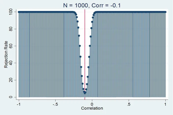
is to infer structural parameters we try a grid search over correlation values. This theorem can help applied researchers in their efforts for inference on structural parameters. Basically, in large samples if the null is true, then at the true correlation level we do not reject the null and all the other values of the correlation we reject the null hypotheses. We can have a very fine grid, and this helps us, as can be seen from Figures 1-2 in simulations.
An important issue in practice is the size distortion of the regular t-test due to the violation of exogeneity. Our test remedies this problem. The key issue is if the null is true, and H0 :β =
values ρ 6= ρ0 can reject the true null. But since we are doing a grid search over correlation
values at ρ = ρ0 6= 0, the test will not reject the null and have the correct inference on the
structural parameters which sets β = β0. The details of the grid over correlation values and
empirics are shown further in this Remark, and Remark 2 below.
To be specific about the implementation of the test, we start with a reasonable value of the correlation between the instrument and the structural error. For example, we can start from -0.3. So at ρ = −0.3 if the absolute value of N T(β0, ρ0) is larger than 1.96, then we do reject
the null, and record this −0.3 as not belonging to true correlation. We repeat this with a grid step of 0.01 in the positive direction. So say that at ρ=−0.1, the absolute value ofN T(β0, ρ0)
is less than 1.96, we record the correlation of -0.1 as belonging to true correlation set. Then we continue this process for other correlation values until maybe a reasonable upper bound is reached in correlation values. More about the details of this grid search is examined in Remark 2 below. The size and power issues will be discussed at length in the Remarks below.
2. What if we miss the true correlation in the grid search when the null hypotheses is true? We know that N T(β0, ρ1) → ∞, and only if we know the true correlation ρ0 we do not reject
the null if it is true. We can pinpoint where the true correlation lies by doing the grid search over the various correlation values and reporting the ones which fail to reject H0.
Observe that the NT test is linear, continuous, and monotonic in the value of the correlation, which is clear from (4). In other words, when we start the grid search from -1, and go toward 1, the NT test will either decrease or increase depending on −sgn(ˆπ). This is good news if we miss the true correlation in our grid search when the null is true.
To illustrate this point assume that the test is -1.96 at correlation 0, and 1.96 at correlation 0.1. Since the test is monotonic and continuous in correlation (ρ), the NT statistic must be equal to each value between -1.96 and 1.96 for some correlation, because of the Intermediate Value Theorem. Therefore, in this example we know that the NT statistics that are evaluated at correlations between 0.0 and 0.1 are less than the 5% critical value, hence the null will not be rejected. So we can get the correct inference, and at the same time since the null is true, we can understand where the true correlation lies (i.e., in this example between 0 and 0.1). The power issue is analyzed in Remarks 6 and 7 below.
3. An important issue here is if the difference between the two-stage least squares estimate and β0 is positive and if the sign of the true correlation is the reverse of the sign of the first stage
test, since the NT will be much larger (see that standard errors will be close since the bias is small). The same issue is true if the difference between the two-stage least squares estimate and
β0 is negative and the sign of the correlation has the same sign of the first stage estimate then
if we reject the null with regular t, we will reject with NT as well. So violation of exogeneity will not change the results of the inference in this case as long as ˆσu is close to ˜σu.
4. Another important point is the local analysis. Assume that β =β0 is true, and consider
what will happen to the test statistic if we use n−1/2
neighborhood of ρ0: ρ0 +d/n 1/2
, where
d 6= 0. In other words, we make a minor mistake in the correlation choice. To state the case rigorously, we call this the local NT test (N Tl(β0, ρ0))
N Tl(β0, ρ0) =
√
n( ˆβ−β0)
˜
σu[|πˆ|−1ˆ Q−zz1/2]
−√nsgn(ˆπ)f(z)(ρ0+d/n 1/2
)
= N T(β0, ρ0)−sgn(ˆπ)f(z)d d
→ N(D,1),
where we use (12), and D=−sgn(ˆπ)f(z)d.
So instead ofN(0,1) distribution as in N T(β0, ρ0) (whereN T(β0, ρ0) assumes that we know
the true correlation level) the true distribution is again normal with variance 1, but shifted to left or right. So this shows that there is local power when we choose the wrong correlation.
Then the question is: can we conduct inference in finite samples with such a minor violation? We answer this question in this remark and Remark 6 below. If β = β0, then two things can happen. First, since we use wrong critical values (i.e., N (0,1) and the truth is N(D,1)), then
N Tl(β0, ρ0) value may be not so large (compared with N T(β0, ρ0)) and still we do not reject the null hypothesis of H0 : β = β0, ρ = ρ0. So this is recorded as non rejection in our grid search
of correlation values. In other words this may enlarge the true correlation set, and we fail to reject the null. But this is good in the sense that the truth is β = β0, and our test still shows
that result.
The second possibility isN Tl(β0, ρ0) is much larger than theN(0,1) critical values and leads
us to reject the null at that specific correlation level (i.e., at ρ0 +d/n1/2
). However, given Remark (2) of Theorem 1, we will detect the true correlation because of monotonicity and the intermediate value theorem, so this problem will not be relevant for inference on β =β0.
∞(when ρ = ρ0). There is power against the fixed alternatives for β at true value of the
correlation (i.e., ρ0).
As an additional fact, when H0 is false, and the true value of β is β1 and if we impose β0,
through Assumptions 1 and 2,
˜
σ2 u−σ
2 u
p
→a <∞,
where a6= 0,
a= (β1−β0) 2
(π2
0Qzz + ΣV V)−2(β1−β0)(π0C+ ΣuV).
Under the alternative the ˜σ2
u is not consistent; however this does not affect the consistency of
the NT statistic when we have fixed alternatives for β.
We now conduct another local power analysis. Set β1 =β0+c/n 1/2
, c 6= 0, note that then
a →0, so ˜σ2 u
p
→σ2 u.
The NT test at the true correlation
√
n( ˆβ−β0)
˜
σu|πˆ|−1ˆ Q−1
zz
− √nsgn(ˆπ)f(z)ρ0−
√
n(β1−β0)
˜
σu|πˆ|−1ˆ Q−1
zz d
→ N(0,1)− c
σu|π0|−1Q−zz1
≡ N(˜c,1),
where ˜c=−c|π0|Qzz/σu.
So we have local power in NT test against local alternatives to β0. This also shows through
˜
c that with strong instruments, the power will be large. Note that with strong instruments, ˜
c (a shift in the mean compared with standard normal) will be large and it will be easy to differentiate the alternative from the null.
6. Next we consider N T(β1, ρ1) and analyze whether it is plausible to have a power loss.
Below we show that this is probable at only implausibly large correlation values when we select strong instruments. The simulations also confirm this.
N T(β1, ρ1) =
√
n( ˆβ−β1)
˜
σu[|πˆ|−1 ˆ Q−zz1/2]
−√nsgn(ˆπ)f(z)ρ1
=
√n( ˆβ
−β0)−√n(β1−β0) ˜
σu[|πˆ|−1Qˆ−1/2
zz ] −
√
nsgn(ˆπ)f(z)ρ0−
√
It is possible then that
√n(β1 −β0) ˜
σu[|πˆ|−1Qˆ−1/2 zz ]
∼
=√nsgn(ˆπ)f(z)(ρ1−ρ0),
where these two terms may be equal to each other and cancel each other in the test statistic. Then N T(β1, ρ1) will not diverge to infinity but converge to a normal distribution. This may result in failure to reject the null. Now we show that with strong instruments, this issue may occur at only implausibly large correlation values. By analyzing the left hand side of the above, and using Estimator of Concentration Parameter= CP :nπˆ2ˆ
Qzz/σ˜2
u we have that:
√
CP(β1−β0)∼=
√
nsgn(ˆπ)f(z)(ρ1−ρ0). (8)
So if the concentration parameter is large, then the possible non-rejection of the false null occurs at correlation values near -1 or +1. These are nearly implausible values in any given application (given that instruments are selected carefully, not randomly). So the problem can be avoided with large n or by using strong instruments.
7. Related to Remark 6 and Remark 2 above, we may have a non-rejection (of the null H0)
region at certain correlation values if ρ1 =ρ0+d/√n, and if the alternative hypotheses is true. This will not be a practical issue as we show. This is related to equation (8) above.
√
CP(β1−β0)∼=sgn(ˆπ)f(z)d. (9)
But this may be avoided with large n or strong instruments, where the left hand and right hand sides will be far apart in (9).
8. Note that if we test at point β0 = ˆβ, ρ0 = 0, then NT takes the value of zero and never
rejects the null. We also see that there is local power at that point with nonzero correlation, to see that
N T(β0 = ˆβ, ρ) = −
√
nsgn(ˆπ)f(z)ρ.
So NT can reject the null with moderate to large n. Also the issue of local power when we impose β0 = ˆβ+a/√n will be analyzed in the exclusion restriction test below.
3.2
The Comparison Between the Regular t and the NT
In the regular t test statistic, we consider H0 : β = β0. In NT we consider the joint null of H0 : β = β0, ρ = ρ0. The joint null is needed, since inference on β depends on the correlation between the structural error and the instrument. The analysis applies to the overidentified case, but to make the comparison easier we demonstrate this using the just identified case. The standard t test, given (k =l = 1), is:
t =
√
n( ˆβ−β0)
ˆ
σu|πˆ|−1ˆ Q−zz1/2
,
where ˆσ2 u =n−
1Pn
i=1(yi−xiβˆ) 2
. The NT at the true correlation is:
N T(β0, ρ0) =
√
n( ˆβ−β0)
˜
σu|πˆ|−1ˆ Q−zz1/2
−√nsgn(ˆπ)f(z)ρ0.
We refer to the test statistic evaluated at (ρ1 6=ρ0) asN T(β0, ρ1). The differences between
the regular and NT are clear from the equations above. First, as discussed above, ˆσu 6= ˜σu,
and they are asymptotically equivalent only in the case of ˆβ →p β0. The second difference is the
subtraction of the drift in the NT. The regular t specifically assumes that ρ0 = 0, the NT does not assume that. When the null is true, β = β0 and ρ= ρ0, our test will always fail to reject.
On the other hand, if β = β1 6= β0, finding the true correlation is not important, since NT is
consistent at all correlation levels, both diverge to infinity and the test rejects.
Since the regular t test assumes ρ0 = 0, if this is not true then under the null t→ ∞. This
is illustrated in the simulation in Table 1. The size distortions with the regular t test are huge, and one can almost always reject the true null. The situation gets worse with larger sample sizes. In the N T(β0, ρ0) test, ρdoes not have to be equal to zero, the test converges to standard
normal distribution, and the test has excellent size (see Tables 2-4) at ρ0.
Then the next question is, ifβ =β0, what if there is a mistake in the true correlation choice
in the NT test? In large samples, there are two possibilities, with a large mistake ρ1 6=ρ0, the
NT test (N T(β0, ρ1) in that case) diverges to infinity as shown in Theorem 1ii. If we have a fine
may reject the null or not depending on the magnitude of the drift. In the regular t ratio, if the true correlation is not 0, but local to some other number, then again the regular t diverges to infinity. So the regular t rejects β = β0 wrongly all the time. Only if the true correlation
is 0 and we put ρ1 = 0 +d/n 1/2
, then the regular t has the same distribution as NT. This is the distribution in Remark 4 after Theorem 1, and Theorem 1 in Berkowitz, Caner, and Fang (2008).
Next, if the null is true, what can we say about the performance of regular t and the NT in finite samples? Here we compare them in a simulation. In Table 1, for n = 100, at 5% nominal size at β0 = 0, regular t rejects the true null 20% at ρ0 = 0.1, and 90% at ρ0 = 0.3. In Table 4,
at β0 = 0, at true ρ0 = 0.1, N T(β0, ρ0) rejects at 5%, and at ρ0 = 0.3N T rejects at 3%. There
is still a very large difference between two. Even if we make a mistake in the choice of true correlation, still NT does better. For example, if we choose a correlation of 0 or 0.2, when the truth is 0.1 the NT rejects the true null at 16-17% compared with 20% rejection of the regular t. At true correlation of 0.3, if we make a mistake and use correlation of 0.2 or 0.4 in our test, the NT rejects at 14-15%, where as the regular t has 90% rejection rate of β0 = 0.
Another issue is that if the regular t fails to reject the true null, is that true for the NT as well? In large samples, regular t test chooses the correct null only when ρ0 = 0, this is true for N T(β0, ρ0) test as well, as is clear from Theorem 1i. In small samples, withn = 100 andρ0 = 0, the size of N T(β0, ρ0) is 4.9% at the nominal 5% level (not shown in Tables). For standard t
test, this is 5.3% as seen in Table 1.
When β =β1 6=β0, both the standard t and the NT are consistent. The NT can have some
power losses in finite samples but the discussion in Remarks 6-7 after Theorem 1 shows that this can be prevented through a choice of strong instruments. Clearly the performance of the NT statistic is far superior to the standard t test statistic.
3.3
The Overidentified Case of One Endogenous Regressor
In this case, since k= 1, l≥k, we assume that
corr(Zim, ui) = cov(Zim, ui)
for all m= 1,· · ·, l. Using Assumption 1 we can rewrite (10) as, for all i= 1,· · ·, n, at the true correlation
Cm =σuqvar(Zim)ρ0. (11)
So with (11) we assume two things in addition to the first case analyzed in section 3.1. First, the instruments are such that cov(Zim, Zip) = 0 for all m 6= p, m = 1,· · ·, l, p = 1,· · ·, l, i = 1,2,· · ·, n. In other words, the instruments are not correlated with each other. In finite samples we can handle this through simple projections as discussed in Remark 2, after Theorem 2. The second assumption in (11) is for all instruments the true correlation between the structural error and the instrument is the same (ρ0). This is similar to regular instrumental variable estimation,
where the claim is that the correlation betweenuiandZimis the same (and 0) for all instruments. So here we extend this assumption to nonzero correlations. Our main results hold with different correlations, but then multiple grid searches would be required. For the many instruments case, this may not be practical. We do not further consider that case here.
Now we construct the test statistic. Note that the former case, (k=l = 1), is a special case of this more general formulation. The following test can be built using Lemma A.1i. The test statistic at the true C is:
√
n( ˆβ−β0−(ˆπ′Qzzˆ πˆ)− 1
ˆ
π′C)
˜
σu(ˆπ′Qzzˆ πˆ)−1/2 . (12)
We can replace the infeasible test in (12) with the following by Assumption 1, (11), and extending (5) to a vector, at true value of the correlation (ρ0),
N T(β0, ρ0) =
√
n( ˆβ−β0−(ˆπ′Qzzˆ πˆ)− 1
ˆ
π′[˜σuqvard(Z
1),· · ·,σu˜ q
d var(Zl)]′ρ
0)
˜
σu(ˆπ′Qzzˆ πˆ)−1/2 ,
where ˜σu is the square root of the estimator ˜σ2
u, and vard(Zm) = 1 n
Pn
i=1(Zim − Zm¯ ) 2
where ¯
Zm =n− 1Pn
i=1Zim for m= 1,· · ·, l. We can further simplify the test above as
N T(β0, ρ0) =
√n( ˆβ
−β0−(ˆπ′Qˆ zzπˆ)−
1
˜
πρ0) ˜
σu(ˆπ′Qzzˆ πˆ)−1/2 , (13)
where ˜π = ˆπ′[˜σuqvard(Z
1),· · ·,σu˜ q
d
var(Zl)]′ which is scalar.
Theorem 2. Under Assumptions 1-2, with (11), and (i). Under the null of H0 :β =β0, ρ=ρ0 when k= 1, l≥k
N T(β0, ρ0) d
→N(0,1).
(ii). Under alternative if β =β0, ρ=ρ1 6=ρ0, then
N T(β0, ρ1)→ ∞.
Remarks.
1. Theorem 2 shows thatN T(β0, ρ0) still has a standard normal distribution whenk = 1, l≥ k. In large samples at the true correlation level the test statistic does not reject the null if H0
is true. At other values of correlation the test rejects the null. In the finite samples, this case is exactly the same as the just identified case. Choosing a fine grid with strong instruments ensures good size and power. If we evaluate at ρ1 6=ρ0 and still do not reject H0 (when β 6=β0
is false), then, as in the just identified case, choosing strong instruments solves the problem. If we evaluate at ρ1 6= ρ0, then our test may reject the true null for that correlation, but this is
easily fixed. Since the test is monotonic in the correlation, choosing a grid and conducting the tests in these new correlation values, we will be able to fail to reject the true null.
2. Note that in finite samples, instruments may be correlated. So we can use the following. Assume that we have two instruments: Zi1, Zi2, for i= 1,· · ·, n. We regress (least squares) Zi1
on Zi2 and define the residual as Zi1⊥. Then we useZi1⊥ and Zi2 in the test.
3.4
The General Case
For testing individual coefficients when k > 1 (multiple endogenous variables) and to get a consistent estimate for σu (i.e., ˜σu) we need to imposeβ =β0 for all parameters. Then we have
a joint NT test for H0 :Rβ =Rβ0, ρ=ρ0, where R is a j ×k matrix. This test will include all
parameters corresponding to endogenous regressors in the structural equation.
So we now introduce the NT evaluated at β0, ρ0 (true correlation). This is constructed in
the same way as before, and the proof is the same, and hence is skipped. Still we impose (11) with Assumption 1
for all m= 1,· · ·, l, i= 1,· · ·, n.
We want to test H0 :Rβ =Rβ0, ρ=ρ0. Define N T(β0, ρ0) ) as follows, by extending (5) to
a vector
N T(β0, ρ0) = n[Rβˆ−Rβ0−R(ˆπ′Qzzˆ πˆ)− 1
ˆ
π′[˜σuqvard(Z
1),· · ·,˜σu q
d var(Zl)]′ρ
0]′
× (Rσ˜2
u(ˆπ′Qzzˆ πˆ)− 1
R′)−1
× [Rβˆ−Rβ0−R(ˆπ′Qzzˆ πˆ)− 1
ˆ
π′[˜σuqvard(Z
1),· · ·,σu˜ q
d var(Zl)]′ρ
0].
Theorem 3. Under Assumptions 1-2, with (14), and (i). Under the joint null of Rβ =Rβ0, ρ=ρ0, we have
N T(β0, ρ0) d
→χ2 j.
(ii). Under the alternative Rβ =Rβ0, ρ=ρ1 6=ρ0,
N T(β0, ρ1)→ ∞.
Remarks.
1.When we use ρ1 (make a mistake in selection of true correlation) then N T(β0, ρ1) → ∞, as in Theorem 1 where ρ1 is used instead of ρ0.
2. The test is consistent with a fixed alternative at β = β1 6= β0. This can be shown easily. With a local alternative, also there is still power if we are at true correlation. When we use correlation values different than the true correlation ρ1 6= ρ0, then it is possible to fail to reject the false null. However, as shown in Remarks 6-7 in the just identified case, using strong instruments solves the problem.
3. Note that with β = β0 and using a correlation value local to ρ0, the test is distributed
as noncentral χ2
in large samples. So the issue is can we still make the correct inference about
β = β0? As explained before, with a fine grid the NT will fail to reject at certain correlation
3.5
Confidence Intervals
Theorems in the previous sections provide us with a way of building joint confidence interval for β0, ρ0. In the multivariate endogenous variables case, start by testing the null of H0 : β =
β0, ρ = ρ0. Then by special case of Theorem 3i (i.e. R = Ik, where Ik is the identity matrix
of dimension k, so the limit in Theorem 3i is χ2
k), we invert the test N T(β0, ρ0), and get the
joint confidence interval. So {(β0, ρ0) :N T(β0, ρ0)≤χ 2
k,α} is an asymptotically valid 100 (1-α)
confidence set, where χ2
k,α represents the 100 α critical value of the χ 2
k distribution.
This also means that the test NT is inverted jointly on a grid search over β0, ρ0 values. To
warn the applied researchers, we do not have a grid only on ρ0 and then use each value of ρ0
to find a confidence interval for β0 based on ˆβ and standard errors. Rather, the grid search is
joint over (β0, ρ0) values. Our test is asymptotically pivotal, and the joint confidence sets show that β0 can be unbounded with positive probability (if we have not normalized covariances as
correlations in Assumption 1, we could have C’s unbounded in the joint confidence set as well). This can be seen from section 3 of Dufour (1997). So the confidence intervals are valid based on inverting the NT statistic. We illustrate the construction of the joint confidence intervals in two empirical examples in Section 5.
Note that related to Remark 8 in the section above ( ˆβ,0) pair is clearly inside the joint confidence interval. This shows that there is a power problem in the test at that specific value.
3.6
Test for Exclusion Restriction
In this part of the paper, we propose a test for the exclusion restriction which can even be used in the just identified case. This is basically testing the null of H0 :β =β0, ρ= 0. So we benefit
from N T(β0,0) where R =Ik. The test is
N T(β0,0) =
n( ˆβ−β0)′(ˆπ′Qzzˆ πˆ)( ˆβ−β0)
˜
σ2 u
.
Corollary 1. Under Assumptions 1-2, with (14), and under the joint null of β =β0, ρ= 0,
we have
N T(β0,0) d
→χ2 k.
Remarks.
1. The proof is a subcase of Theorem 3, and hence it is skipped.
2. The implementation is as follows. First setup a plausible grid values for β0, a compact
interval of [β0l, β0u], where β0l, β0u represent the lower and upper bound of plausible β0 values.
With these values we test N T(β0,0). If for all plausible values the test rejects the null, then the
instruments are not exogenous.
3. Note that this test is even valid for k = l, which is the just identified case. To our knowledge this is the first test statistic to do so in the literature.
4. The intuition of the test is such that by keeping ρ0 = 0, and changing β0 values in the
test, we assume if the model is true, we find such β0 andρ0 = 0, so the null will not be rejected.
But if the instruments are not exogenous, the test will be rejected at all grid values for β0.
5. Regular t and Wald tests for testing only β =β0 are very similar in form, the difference
being the ˜σ2
u. Previous literature such as Berkowitz, Caner and Fang (2008) already found that
even with a minor violation of exogeneity, the distributions change and there is a drift which depends on the correlation between the instrument and the error. So in one sense, we are benefiting from that idea here. Instead of fixing β0 to be tested once, we test over grid values
of β0. If all of them reject the null then the instruments are not exogenous.
6. Note that the test at two stage least squares estimate (i.e. when we impose β0 = ˆβ) will
never reject the null. So there is a power problem at that point. But we also see that when we have β0 = ˆβ+a/√n, where a is a vector of non zero-constants
N T(β0,0) =
a′(ˆπ′Qzzˆ πˆ)a
˜
σ2 u
.
Then there will be local power with strong instruments, since the Concentration Parameter estimate is nπˆ′Qzzˆ π/ˆ ˜σ2
4
Simulation
In this part of the paper we conduct simulations to answer the following questions. First, can we verify the results of Theorem 1? Namely, can we see that N T(β0, ρ0)
d
→ N(0,1), and
N T(β0, ρ1) → ∞ in large samples? The second issue is the finite sample behavior of the test
statisticN T(β0, ρ0). In the finite samples given a grid search (it may be a very fine grid search,
with very small steps in a given empirical application), does the smallest rejection level still correspond to N T(β0, ρ0)?. The third question is related to power of the test. Is there a power
loss at certain grid points as discussed after Theorem 1? If there is, can we also see that they are near extreme correlation values for a given application? If this power loss occurs away from [-0.3, 0.3] range of correlations, then that power loss may not be important as it will not arise in practice with reasonably chosen instruments. We generate the data with one instrument (l= 1), one endogenous regressor (k= 1) and no control variables.
yi =Xiβ0+ui, (15)
Xi =Ziπ0+Vi, (16)
where β0 = 0 , i = 1,· · ·, n, and π0 = 2. The structural error ui, the first stage error Vi,
and the instrument are iid. These are generated from the same joint normal distribution with
N(0,Λ), where
Λ =
1 cov(Zi, ui) 0
cov(Zi, ui) 1 cov(Vi, ui) 0 cov(ui, Vi) 1
,
since varZi = 1, varui = 1, cov(Zi, ui) is also the correlation between Zi, ui. This is denoted as ρ0 in the other sections. The covariance between Vi, ui is set at 0.5. Since the variances are
set at 1, the true correlation between the structural error and the instrument varies among -0.5, -0.3, -0.1, 0.1, 0.3, 0.5. The grid step is 0.1 for the tables. For the graphs the true correlation is set at -0.1 and the grid step is 0.01.1
The sample sizes in the tables are n = 100,200,1000. The iteration number is 10000. For the size exercise, we report the percentage of rejections at 5% critical values from the standard normal distribution (-1.96, +1.96).
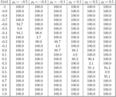
Table 2 provides the size ofN T(β0, ρ0) and the rejection rate of the true nullH0 :β= 0, ρ= ρ0 for N T(β0, ρ1) (tests evaluated at ρ1 6= ρ0) at n = 1000. In Table 2, ρ0 represents the true
correlation between the structural error (ui) and the instrument (Zi). The first column is the grid values of the correlation “Grid”. When the grid value is equal toρ0 then the size of the test
should be 5% at that level ideally. Otherwise if the grid value of the correlation is not equivalent to ρ0 then the rejection rate of the test should be near 100% according to Theorem 1ii. We
see that the results in Table 2 confirm Theorem 1. Namely, the size of the N T(β0, ρ0) test is
at the 1-5% level (i.e., at ρ0 = −0.5, N T(β0, ρ0) is the one that corresponds to Grid =−0.5).
Otherwise whenGrid=ρ1 6=ρ0 the test isN T(β0, ρ1). When we look at theN T(β0, ρ1) test the
rejection rate is 88-100% at the 5% nominal level. So if we have a grid search of the correlation, then only at the true value we will get the 5% rejection at nominal levels, otherwise we almost always reject the null. In that sense, we can differentiate the true correlation by looking at the absolute value of the NT statistic. If the absolute value of the test is less than 1.96 then the test fails to reject and the correlation that is used belongs to true correlation set.
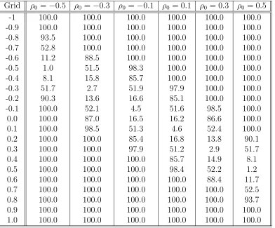
To see how reliable this is in finite samples, we conduct the same exercise withn= 100, n = 200 observations. In Tables 3 - 4 we see that N T(β0, ρ0) test achieves 1-5% size at 5% nominal level. This confirms that even in the finite samples the asymptotic approximation is very good. Table 3 shows the size of the test for N T(β0, ρ0) and the rejection rate of the true null for
N T(β0, ρ1) at n = 200. For example, at true correlation of ρ0 = −0.1, theN T(β0, ρ0) has the
size of 4.5%, and N T(β0, ρ1) (which imposes ρ1 = −0.2) has the the rejection rate of 29.6% when the true null is β = 0, ρ = −0.1. But still there is substantial rejection rate difference between N T(β0, ρ1) and N T(β0, ρ0) tests. At n = 100 in Table 4, N T(β0, ρ0) still has the smallest rejection rate. Tables 3-4 support our claim in Remarks 2 and 4 (in the just identified case) of the existence of a region of non-rejection of the true null when the null ofβ = 0, ρ=ρ0
is true. This region is around the true correlation value. We also report size results with a much finer grid of 0.01, these are shown in Figures 1 and 2, and verify Theorem 1.
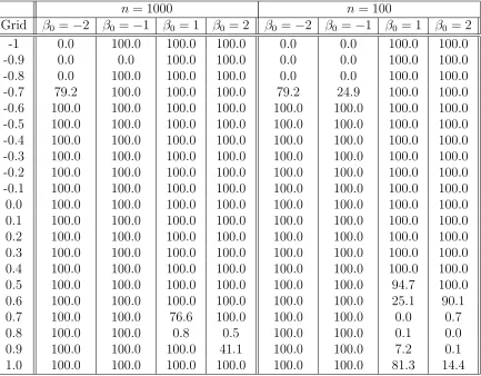
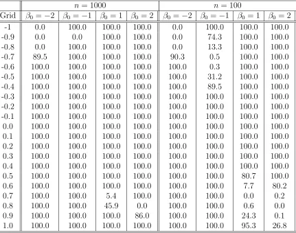
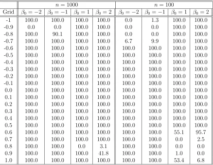
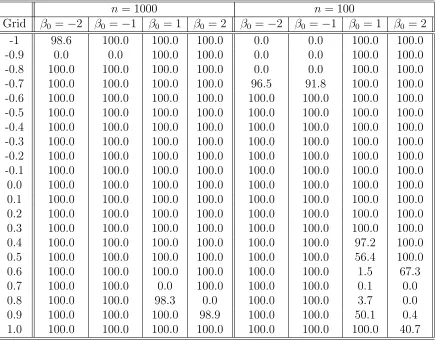
Tables 5-8, report the percentage of the rejections when true β is not equal to zero. We have the same number of iterations as the size exercise, and the same critical values are used. The true values of β0 = −2,−1,1,2, and we test H0 : β = 0, ρ = ρ0, and n = 100,1000. The
results confirm the remarks after Theorem 1. Namely, the power of N T is very good at almost all the relevant correlation levels for applications. Even at alternate correlation values (using
concentration parameter estimate by putting π = 5, and this gives much better power results. We also experiment with β0 =−0.5,−0.3,0.3,0.5, the results are very similar even in this close
neighborhood of 0. These are not reported.
The applied researcher may use this method for a grid of correlations, ρ, between [-0.3, 0.3] for NT test. If one finds a region of non-rejection of the null, then this is also the confidence interval. If the grid search shows only rejection of the null, then the alternative is true. This test is a significant improvement to the regular t, which does not test the joint null and falsely rejects when ρ6= 0.
In this simulation section, we also have size and power results for the exclusion restriction that is introduced. We test the joint null of H0 : β = β0, ρ = 0. We use the setup (15)(16),
with the same covariance structure Λ. For the size part of the test we set β0 = 0, ρ0 = 0, and
we evaluate N T(0,0). If the test is larger than the 5% crtical value of χ2
1 the we reject the null.
There are 10000 iterations used. The sample size varies between 100, 200, 300, 1000. We record the percentage of the rejections of the true null. The results are in Table 9. It is clear that at all sample sizes the size is very good, and very close to 5%. So the exclusion restriction test has no size issue. The next issue is the power of the test. For this we propose two power tables. In this exercise (Table 10) the true model is β0 = 0, ρ0 6= 0. However, the test imposesβ = 0, ρ= 0. In
this power exercise, ρ0 =−0.5,−0.3,−0.1,0.1,0.3,0.5. Again we record percentage of rejection of the null. This is done at 5% level for χ2
1 distribution. We observe two things. If we have the
correlation as -0.3 or 0.3, the test has very good power regardless of the sample size (87-100%). But if ρ0 = 0.1, the exclusion restriction test has 16% power at n = 100. With n = 1000, the
power increases to 88%. So large samples make a big difference if the true correlation is nonzero but close to zero. In the second power Table (Table 11), the true null is ρ0 = 0, but β0 6= 0.
And still we imposeβ = 0, ρ= 0. The results are similar to the Table 10. The power declines at
n = 100 when the structural parameter is nonzero but close to the zero, but with large samples, we can reject the null with probability one.
5
Implementation and Empirical Examples
The next step is to calculate N T(β0, ρ0) by iterating over potential values in a nested loop.
attention here to the range [-0.3, 0.3]. From the simulation results we find the statistic suffers from a loss of power at the extreme values of correlation. Since most instruments are carefully chosen, [-0.3, 0.3] is a reasonable range in practice. The range of β0 to test depends on the
economic environment that dictates reasonable effect sizes and also what inferences the applied researcher chooses to draw.
If our interest centers on significance testing, then testingH0 :β0 = 0, ρ=ρ0 is a reasonable
choice. In that case, if the applied researcher finds that the absolute value of N T drops below 1.96 in absolute value within a reasonable range of correlation values, then we fail to reject the null. On the other hand, if the researcher finds that the N T yields rejection at all reasonable levels of the grid, we can confidently reject the null and interpret the structural coefficient as being non-zero.
5.1
Empirical Examples
We apply our technique to two empirical examples. First, we replicate the results from Acemoglu and Johnson (2005), hereafter AJ. As discussed in the introduction, the main results in AJ utilize early settler mortality to instrument for institutions when measuring the effect of institutions on economic growth as measured by GDP per capita. For our study, we have obtained the data used by AJ on 64 countries. In this discussion we focus on Table 2 of AJ which provides estimates for the just identified case of one instrument and one endogenous variable. In Table 2, Panel C, Column (3) of AJ, the two-stage least squares estimate of the effect of the constraint on executive power on GDP per capita is 0.756 with a standard error of 0.146. This coefficient is interpreted as highly statistically significant under standard inference.
Figure 3 presents a graphical depiction of the N T for reasonable grid values. The black region indicates combinations of β0, ρ0 that cannot be rejected. This region can be interpreted as a confidence interval for the joint values of β0, ρ0. Notice that within the range [-0.30, +0.30] N T indicates rejection for β0 = 0. The regions of non-rejection are bounded away fromβ0 = 0 and demonstrate that, in fact, β0 > 0. Note that even if ρ0 6= 0 we can still infer that β0 > 0.
Because the region of non-rejection includes ρ0 = 0, the exclusion restriction test indicates that the we cannot reject perfect exogeneity in this example.
educational attainment.2
This paper finds much larger returns to education relative to previous work. As in AJ, the instrumental variable in Card (1995) may not be completely exogenous, leading to biased results.
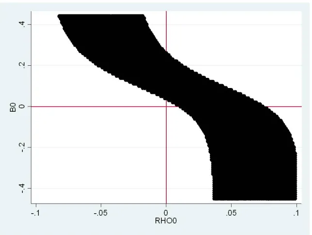
Figure 4 presents a graphical depiction of the N T for small correlation values near the origin. Again, the black region indicates combinations of β0, ρ0 that cannot be rejected. Note
that in this case, the region of non-rejection is unbounded both above and below. Therefore, the confidence interval for β must include all possible values and no inference can be drawn. Notice again that the origin (β0 = 0, ρ0 = 0) is not part of the non-rejected region. In fact, N T(0,0) = 2.33. Under naive testing, this test statistic could be erroneously interpreted as indicating β 6= 0. But, as the figure demonstrates, when considering the joint null it is clear that without also considering ρ one could draw incorrect inferences from rejection at β0 = 0.
We see here that there is not enough information to identify β and we cannot reject that ρ is in the interval [−.1, .1]. The exclusion restriction test again indicates that for some values ofβ0
one cannot reject that ρ0 = 0. Therefore, we cannot reject that the instrument is valid.
6
Discussion and Conclusion
In this paper we tackle one of the most important problems in applied econometrics, the violation of the exclusion restriction in instrumental variables (IV) estimation. We recognize that to infer anything about the structural parameters, one must know the correlation between the error and the instruments. Regular inference techniques assume that this correlation is zero. In any application this is a strong and likely incorrect assumption. We propose a joint test of structural parameters together with the correlation parameter. Since the correlation cannot be estimated in the test statistic that we develop, we conduct a grid search. This test corrects the bias in the two stage least squares estimators. Also we show that joint confidence intervals for β0, ρ0 can be built by inverting this test statistic.
In future research, we want to extend these results to other contexts such as nonlinear GMM and possibly identification robust tests.
2The data set used in Card (1995) is available on David Card’s website at:
REFERENCES
Acemoglu, Daron, Simon Johnson, and James A. Robinson (2001), “The Colonial Origins of Com-parative Development: An Empirical Investigation,”American Economic Review, 91, 1369-1401. Acemoglu, Daron and Simon Johnson (2006), “Unbundling Institutions,”Journal of Political
Econ-omy, 113, 949-995.
Angrist, Joshua D. (1990), “Lifetime Earnings and the Vietnam Era Draft Lottery: Evidence from Social Security Administrative Records,” American Economic Review, 80, 313-336.
Angrist, Joshua D. and Alan B. Krueger (1991), “Does Compulsory School Attendance Affect Schooling and Earnings,” Quarterly Journal of Economics, 106, 979-1014.
Ashley, Richard, (2009), “Assessing the Credibility of Instrumental Variables Inference with Im-perfect Instruments via Sensitivity Analysis,” Journal of Applied Econometrics, Feb, 2009, Vol. 24: 325-337.
Berkowitz, Daniel, Mehmet Caner, and Ying Fang (2008), “Are nearly exogenous instruments reliable?” Economics Letters, 101, 202-23.
Berkowitz, Daniel, Mehmet Caner, and Ying Fang (2009), “The Validity of Instruments Revisited” Working paper, Dept. of Economics, North Carolina State University.
Caner, Mehmet, (2009) ”Near Exogeneity and Weak Identification in Generalized Empirical Like-lihood Estimators: Many Moment Asymptotics,” Working paper, Department of Economics, North Carolina State University.
Card, David (1995), “Using Geographic Variation in College Proximity to Estimate the Returns to Schooling,” in Aspects of Labour Market Behaviour: Essays in Honor of John Vanderkamp, eds. L. N. Christofides et al. Toronto: University of Toronto Press. 201-221.
Conley, Tim, Carsten Hansen, Peter Rossi (2007), ”Plausibly Exogenous”, Unpublished manuscript. Booth School of Business, University of Chicago.
Djankov, Simeon, Rafael La Porta, Florencio Lopez-de-Silanes and Andrei Shleifer (2003), “Courts,”
Quarterly Journal of Economics, 118, 453-517.
Duflo, Esther (2001), “Schooling and Labor Market Consequences of School Construction in In-donesia: Evidence from an Unusual Policy Experiment,” American Economic Review, Vol. 91(4), pages 795-813, September.
Dufour, Jean-Marie (1997), ”Some Impossibility Theorems in Econometrics with Applications to Structural and Dynamic Models,” Econometrica, vol.65, 1365-1389.
Glaeser, Edward, Rafael La Porta, Florencio Lopez-de-Silanes and Andrei Shleifer (2004), “Do Institutions Cause Growth?” Journal of Economic Growth, 9, 271-303.
Guggenberger, Patrik, (2009), ”On the Asymptotic Size Distortion of tests when instruments locally violate the exogeneity assumption,” Working paper, Department of Economics, UCLA. Guiso, Luigi, Paola Sapienza and Luigi Zingales (2006), “Does Culture Affect Economic
Out-comes,” Journal of Economic Perspectives, vol. 20(2), pages 23-48, Spring.
Hall, Robert E. and Charles I. Jones (1999), “Why Do Some Countries Produce So Much More Output per Worker than Others?” Quarterly Journal of Economics, 114, 83-116.
Kray, A. (2008) ”Instrumental Variables Regression with Honestly Uncertain Exclusion Restric-tions,” unpublished manuscript. World Bank.
Mauro, Paolo (1995), “Corruption and Growth,”Quarterly Journal of Economics, 110, 681-712. Meghir, Costas and Marten Palme (2005), “Assessing the Effect of Schooling on Earnings Using a
Social Experiment,” American Economic Review, March 2005, pp 414-424.
Figure 1: Simulation results for N=100 when the correlation is -0.1
[image:30.612.126.478.462.697.2]Figure 3: Example Using Acemoglu and Johnson (2005)
[image:31.612.141.463.456.699.2]Table 1: Size (5% level), Standard t test
ρ0 = −0.5 −0.3 −0.1 0 0.1 0.3 0.5 n= 1000 100.0 100.0 87.9 5.3 88.8 100.0 100.0
n= 200 100.0 99.0 26.9 5.3 32.9 99.2 100.0
n= 100 100.0 85.2 15.4 5.3 19.9 89.6 99.9
Note: ρ0 represents the true correlation between the single instrument and the error (second
stage equation). The first column header is true correlation, all the other column headers are specific true correlation values.
Table 2: Rejection Rate of The Null β0 = 0, ρ=ρ0, N T(β0, ρ0), N T(β0, ρ1) n = 1000
Grid ρ0 =−0.5 ρ0 =−0.3 ρ0 =−0.1 ρ0 = 0.1 ρ0 = 0.3 ρ0 = 0.5
-1 100.0 100.0 100.0 100.0 100.0 100.0 -0.9 100.0 100.0 100.0 100.0 100.0 100.0 -0.8 100.0 100.0 100.0 100.0 100.0 100.0 -0.7 100.0 100.0 100.0 100.0 100.0 100.0 -0.6 94.7 100.0 100.0 100.0 100.0 100.0 -0.5 0.8 100.0 100.0 100.0 100.0 100.0 -0.4 94.1 90.8 100.0 100.0 100.0 100.0 -0.3 100.0 3.7 100.0 100.0 100.0 100.0 -0.2 100.0 90.0 88.7 100.0 100.0 100.0 -0.1 100.0 100.0 4.8 100.0 100.0 100.0 0.0 100.0 100.0 88.7 88.1 100.0 100.0 0.1 100.0 100.0 100.0 4.9 100.0 100.0 0.2 100.0 100.0 100.0 88.2 90.4 100.0 0.3 100.0 100.0 100.0 100.0 3.1 100.0 0.4 100.0 100.0 100.0 100.0 91.4 94.4 0.5 100.0 100.0 100.0 100.0 100.0 0.9 0.6 100.0 100.0 100.0 100.0 100.0 95.1 0.7 100.0 100.0 100.0 100.0 100.0 100.0 0.8 100.0 100.0 100.0 100.0 100.0 100.0 0.9 100.0 100.0 100.0 100.0 100.0 100.0 1.0 100.0 100.0 100.0 100.0 100.0 100.0
Note: Grid represents the grid correlation values that we put into the NT tests. WhenGrid =ρ0,
the we have N T(β0, ρ0) test, otherwise the tests are N T(β0, ρ1). The critical values are -1.96,
+1.96. We set π0 = 2. For example, in column 2, ρ0 = −0.5, when Grid = −0.5, the test is
[image:32.612.110.495.325.647.2]Table 3: Rejection Rate of The Nullβ0 = 0, ρ=ρ0, N T(β0, ρ0), N T(β0, ρ1)n = 200
Grid ρ0 =−0.5 ρ0 =−0.3 ρ0 =−0.1 ρ0 = 0.1 ρ0 = 0.3 ρ0 = 0.5
-1 100.0 100.0 100.0 100.0 100.0 100.0 -0.9 100.0 100.0 100.0 100.0 100.0 100.0 -0.8 100.0 100.0 100.0 100.0 100.0 100.0 -0.7 88.8 100.0 100.0 100.0 100.0 100.0 -0.6 24.0 100.0 100.0 100.0 100.0 100.0 -0.5 1.1 83.4 100.0 100.0 100.0 100.0 -0.4 22.7 27.0 99.0 100.0 100.0 100.0 -0.3 86.5 3.1 80.9 100.0 100.0 100.0 -0.2 100.0 26.4 28.9 98.9 100.0 100.0 -0.1 100.0 82.8 4.9 80.7 100.0 100.0 0.0 100.0 100.0 29.5 28.0 100.0 100.0 0.1 100.0 100.0 80.8 4.5 82.1 100.0 0.2 100.0 100.0 98.8 29.1 27.5 100.0 0.3 100.0 100.0 100.0 81.4 3.0 86.2 0.4 100.0 100.0 100.0 100.0 27.8 22.4 0.5 100.0 100.0 100.0 100.0 83.4 1.0 0.6 100.0 100.0 100.0 100.0 100.0 24.3 0.7 100.0 100.0 100.0 100.0 100.0 89.2 0.8 100.0 100.0 100.0 100.0 100.0 100.0 0.9 100.0 100.0 100.0 100.0 100.0 100.0 1.0 100.0 100.0 100.0 100.0 100.0 100.0
Note: Grid represents the grid correlation values that we put into the NT tests. WhenGrid =ρ0,
the we have N T(β0, ρ0) test, otherwise the tests are N T(β0, ρ1). The critical values are -1.96,
+1.96. We set π = 2. For example, in column 2, ρ0 = −0.5, when Grid = −0.5, the test is
Table 4: Rejection Rate of The Nullβ0 = 0, ρ=ρ0, N T(β0, ρ0), N T(β0, ρ1)n = 100
Grid ρ0 =−0.5 ρ0 =−0.3 ρ0 =−0.1 ρ0 = 0.1 ρ0 = 0.3 ρ0 = 0.5
-1 100.0 100.0 100.0 100.0 100.0 100.0 -0.9 100.0 100.0 100.0 100.0 100.0 100.0 -0.8 93.5 100.0 100.0 100.0 100.0 100.0 -0.7 52.8 100.0 100.0 100.0 100.0 100.0 -0.6 11.2 88.5 100.0 100.0 100.0 100.0 -0.5 1.0 51.5 98.3 100.0 100.0 100.0 -0.4 8.1 15.8 85.7 100.0 100.0 100.0 -0.3 51.7 2.7 51.9 97.9 100.0 100.0 -0.2 90.3 13.6 16.6 85.1 100.0 100.0 -0.1 100.0 52.1 4.5 51.6 98.5 100.0 0.0 100.0 87.0 16.5 16.2 86.6 100.0 0.1 100.0 98.5 51.3 4.6 52.4 100.0 0.2 100.0 100.0 85.4 16.8 13.8 90.1 0.3 100.0 100.0 97.9 51.2 2.9 51.7 0.4 100.0 100.0 100.0 85.7 14.9 8.1 0.5 100.0 100.0 100.0 98.4 52.2 1.2 0.6 100.0 100.0 100.0 100.0 88.4 11.7 0.7 100.0 100.0 100.0 100.0 100.0 52.5 0.8 100.0 100.0 100.0 100.0 100.0 93.7 0.9 100.0 100.0 100.0 100.0 100.0 100.0 1.0 100.0 100.0 100.0 100.0 100.0 100.0
Note: Grid represents the grid correlation values that we put into the NT tests. WhenGrid =ρ0,
the we have N T(β0, ρ0) test, otherwise the tests are N T(β0, ρ1). The critical values are -1.96,
+1.96. We set π = 2. For example, in column 2, ρ0 = −0.5, when Grid = −0.5, the test is
Table 5: Rejection percentage of H0 :β= 0, ρ0 = 0.1, N T(β, ρ0), N T(β, ρ1)
n = 1000 n= 100
Grid β0 =−2 β0 =−1 β0 = 1 β0 = 2 β0 =−2 β0 =−1 β0 = 1 β0 = 2
-1 0.0 100.0 100.0 100.0 0.0 0.0 100.0 100.0 -0.9 0.0 0.0 100.0 100.0 0.0 0.0 100.0 100.0 -0.8 0.0 100.0 100.0 100.0 0.0 0.0 100.0 100.0 -0.7 79.2 100.0 100.0 100.0 79.2 24.9 100.0 100.0 -0.6 100.0 100.0 100.0 100.0 100.0 100.0 100.0 100.0 -0.5 100.0 100.0 100.0 100.0 100.0 100.0 100.0 100.0 -0.4 100.0 100.0 100.0 100.0 100.0 100.0 100.0 100.0 -0.3 100.0 100.0 100.0 100.0 100.0 100.0 100.0 100.0 -0.2 100.0 100.0 100.0 100.0 100.0 100.0 100.0 100.0 -0.1 100.0 100.0 100.0 100.0 100.0 100.0 100.0 100.0 0.0 100.0 100.0 100.0 100.0 100.0 100.0 100.0 100.0 0.1 100.0 100.0 100.0 100.0 100.0 100.0 100.0 100.0 0.2 100.0 100.0 100.0 100.0 100.0 100.0 100.0 100.0 0.3 100.0 100.0 100.0 100.0 100.0 100.0 100.0 100.0 0.4 100.0 100.0 100.0 100.0 100.0 100.0 100.0 100.0 0.5 100.0 100.0 100.0 100.0 100.0 100.0 94.7 100.0 0.6 100.0 100.0 100.0 100.0 100.0 100.0 25.1 90.1 0.7 100.0 100.0 76.6 100.0 100.0 100.0 0.0 0.7 0.8 100.0 100.0 0.8 0.5 100.0 100.0 0.1 0.0 0.9 100.0 100.0 100.0 41.1 100.0 100.0 7.2 0.1 1.0 100.0 100.0 100.0 100.0 100.0 100.0 81.3 14.4
Note: Grid represents the grid correlation values that we put into the NT tests. Whenρ0 =Grid, then we have N T(β, ρ0) test, otherwise the tests are N T(β, ρ1). The critical values are -1.96,
Table 6: Rejection percentage of H0 :β= 0, ρ0 =−0.1, N T(β, ρ0), N T(β, ρ1)
n = 1000 n= 100
Grid β0 =−2 β0 =−1 β0 = 1 β0 = 2 β0 =−2 β0 =−1 β0 = 1 β0 = 2
-1 0.0 100.0 100.0 100.0 0.0 100.0 100.0 100.0 -0.9 0.0 0.0 100.0 100.0 0.0 74.3 100.0 100.0 -0.8 0.0 100.0 100.0 100.0 0.0 13.3 100.0 100.0 -0.7 89.5 100.0 100.0 100.0 90.3 0.5 100.0 100.0 -0.6 100.0 100.0 100.0 100.0 100.0 0.3 100.0 100.0 -0.5 100.0 100.0 100.0 100.0 100.0 31.2 100.0 100.0 -0.4 100.0 100.0 100.0 100.0 100.0 89.5 100.0 100.0 -0.3 100.0 100.0 100.0 100.0 100.0 100.0 100.0 100.0 -0.2 100.0 100.0 100.0 100.0 100.0 100.0 100.0 100.0 -0.1 100.0 100.0 100.0 100.0 100.0 100.0 100.0 100.0 0.0 100.0 100.0 100.0 100.0 100.0 100.0 100.0 100.0 0.1 100.0 100.0 100.0 100.0 100.0 100.0 100.0 100.0 0.2 100.0 100.0 100.0 100.0 100.0 100.0 100.0 100.0 0.3 100.0 100.0 100.0 100.0 100.0 100.0 100.0 100.0 0.4 100.0 100.0 100.0 100.0 100.0 100.0 100.0 100.0 0.5 100.0 100.0 100.0 100.0 100.0 100.0 80.7 100.0 0.6 100.0 100.0 100.0 100.0 100.0 100.0 7.7 80.2 0.7 100.0 100.0 5.4 100.0 100.0 100.0 0.0 0.2 0.8 100.0 100.0 45.9 0.0 100.0 100.0 0.6 0.0 0.9 100.0 100.0 100.0 86.0 100.0 100.0 24.3 0.1 1.0 100.0 100.0 100.0 100.0 100.0 100.0 95.3 26.8
Note: Grid represents the grid correlation values that we put into the NT tests. Whenρ0 =Grid, then we have N T(β, ρ0) test, otherwise the tests are N T(β, ρ1). The critical values are -1.96,
Table 7: Rejection percentage of H0 :β = 0, ρ0 = 0.3,N T(β, ρ0), N T(β, ρ1)
n = 1000 n= 100
Grid β0 =−2 β0 =−1 β0 = 1 β0 = 2 β0 =−2 β0 =−1 β0 = 1 β0 = 2
-1 100.0 100.0 100.0 100.0 0.0 1.3 100.0 100.0 -0.9 0.0 0.0 100.0 100.0 0.0 0.0 100.0 100.0 -0.8 100.0 90.1 100.0 100.0 0.0 0.0 100.0 100.0 -0.7 100.0 100.0 100.0 100.0 6.7 9.9 100.0 100.0 -0.6 100.0 100.0 100.0 100.0 100.0 100.0 100.0 100.0 -0.5 100.0 100.0 100.0 100.0 100.0 100.0 100.0 100.0 -0.4 100.0 100.0 100.0 100.0 100.0 100.0 100.0 100.0 -0.3 100.0 100.0 100.0 100.0 100.0 100.0 100.0 100.0 -0.2 100.0 100.0 100.0 100.0 100.0 100.0 100.0 100.0 -0.1 100.0 100.0 100.0 100.0 100.0 100.0 100.0 100.0 0.0 100.0 100.0 100.0 100.0 100.0 100.0 100.0 100.0 0.1 100.0 100.0 100.0 100.0 100.0 100.0 100.0 100.0 0.2 100.0 100.0 100.0 100.0 100.0 100.0 100.0 100.0 0.3 100.0 100.0 100.0 100.0 100.0 100.0 100.0 100.0 0.4 100.0 100.0 100.0 100.0 100.0 100.0 100.0 100.0 0.5 100.0 100.0 100.0 100.0 100.0 100.0 100.0 100.0 0.6 100.0 100.0 100.0 100.0 100.0 100.0 55.1 95.7 0.7 100.0 100.0 100.0 100.0 100.0 100.0 0.0 2.5 0.8 100.0 100.0 0.0 3.1 100.0 100.0 0.0 0.0 0.9 100.0 100.0 100.0 41.8 100.0 100.0 1.0 0.0 1.0 100.0 100.0 100.0 100.0 100.0 100.0 53.4 6.8
Note: Grid represents the grid correlation values that we put into the NT tests. Whenρ0 =Grid, then we have N T(β, ρ0) test, otherwise the tests are N T(β, ρ1). The critical values are -1.96,