On the Trade-off between Power Consumption and Time
Synchronization Quality for Moving Targets under
Large-Scale Fading Effects in Wireless Sensor Networks
Pablo Briff1, Leonardo Rey Vega2, Ariel Lutenberg1, Fabian Vargas3 1
Embedded Systems Laboratory, Faculty of Engineering, University of Buenos Aires, Argentina
2
Signal Processing and Communications Laboratory, Faculty of Engineering, University of Buenos Aires, Argentina
3
Signals and Systems for Computing Group, Faculty of Engineering, Catholic University, PUCRS, Brazil Email: [email protected], [email protected], [email protected], [email protected]
Received May 2013
ABSTRACT
In this work we find a lower bound on the energy required for synchronizing moving sensor nodes in a Wireless Sensor Network (WSN) affected by large-scale fading, based on clock estimation techniques. The energy required for synchro- nizing a WSN within a desired estimation error level is specified by both the transmit power and the required number of messages. In this paper we extend our previous work introducing nodes’ movement and the average message delay in the total energy, including a comprehensive analysis on how the distance between nodes impacts on the energy and synchronization quality trade-off under large-scale fading effects.
Keywords: Wireless Sensor Networks; Clock Offset Estimation; Time Synchronization; Wireless Channel Fading; Moving Targets
1. Introduction
With the advent of wireless technologies over the last decade, Wireless Sensor Networks (WSN’s) are over-taking wired networks in the field of sensing [1]. A WSN typically consists of low cost battery-powered or self- powered sensor nodes. Thus, energy management be- comes a substantial matter in order to guarantee reasona- ble sensors’ lifetime values. Time synchronization algo-rithms aim to provide mechanisms for nodes to obtain an estimate of their internal clocks with respect to the other nodes, aiming to reach a consensus on the concept of time among all the nodes. For each node i, its internal clock ci can be modeled as a linear equation with a
corresponding skew αi and offset βi [2,3], namely
( )
i i i
c t = +α β . In order to achieve a target synchroniza-tion quality, parameter estimasynchroniza-tion techniques can be ap-plied, being the estimation error a function of the estimator and the number of samples employed. Time synchronization can be energy-consuming since it in- volves wireless messages exchange, however, when achieved, it allows significant energy savings through network power management. In all, WSN synchroniza- tion remains amongst the most challenging open topics in WSN’s [4]. In our previous work [5] we had introduced the existing tradeoff between time synchronization accu-
racy and synchronization energy, although we did not contemplate nodes’ movement in our analysis. In this paper we introduce this important feature under large-scale fad- ing, a situation that is present in a realistic environment where nodes change their relative distance within a network.
2. Related Work
tained as follows [8]:
2 2
( ) 1
2 2
1 1
ˆ
var( )
( )
m i
BP i
offset m m
i i
i i
D
m D D
σ
θ =
= =
≥
−
∑
∑
∑
(1)
From (1), the estimation quality (variance of the clock offset estimator) depends on the number of received mes-sages m and the time stamps differences Di.
Increas-ing m will enhance estimation quality in detriment of the energy consumed. While many authors expose this energy-synchronization quality balance as a known open topic (such as [9,10]), to the best of our knowledge, pre- vious contributions in the field of clock synchronization focus on the algorithmic aspect of the timing mechanism with little concern on the energy and delay required to attain such a goal. In [11], authors propose a mechanism for synchronizing a WSN by means of constructive in-terference in order to achieve low duty cycles in radio operation, thus minimizing the energy spent, although they do not mention the existing trade-off between ener-gy and synchronization accuracy. In [12], the authors ex-pose the trade-off of energy consumption and synchroni-zation quality from a local sleep-time perspective, with-out contemplating the energy spent in nodes interaction. Also, [13] aims to minimize the energy for maximum accuracy but from a local node’s perspective, with low duty cycle and low frequency crystal oscillators hardware. More recent works such as [11,14] approach the energy efficiency problem from a protocol perspective, without detailing the physical phenomena involved in wireless channels. For example, [14] proposes a new algorithm, the Recursive Time Synchronization Protocol (RTSP), which aims to minimize the number of transmitted mes-sages in a WSN, although the authors do not include in their analysis either transmit or receive power in each sensor node as part of the minimization problem. There- fore, the tradeoff “power consumption-clock synchroni- zation quality” is a critical issue for wireless embedded systems that requires finding an optimal solution.
3. One-Way Message Clock Offset
Estimation Quality as a Function of
Transmit Power
3.1. Motivation
We will use one-way message mechanism as the starting point for exposing the underlying issues associated with clock synchronization by means of wireless messages. The Flooding Time Synchronization Protocol [15] uses this technique to estimate the sender’s clock offset through a linear regression of the received samples.
3.2. Model Statement
Transmit power and clock synchronization quality oper-ate on different layers: the first one is a physical magni-tude whereas the latter belongs to the application layer. However, prior to estimation, physical layer reception oc-curs with a given probability of failure as a function of the transmit power S, given by the channel’s outage prob-ability Pout, defined as the probability that the received
signal falls under a minimum acceptable threshold [16]. Let’s consider each node’s clock offset θ is estimated with an unbiased estimator ˆθ and let σθ2ˆ be the
va-riance of the clock offset estimator. Consider sender node
A sends m packets while receiver node B receives
[ ] (1 out)
m =E M = ⋅ −m P successful messages, where M
is a binomial random variable, i.e. M ~ ( ,1b m −Pout). The average delay per message can also be derived as a function of the outage probability as follows:
1
M M
out T m T
m P
δ = ⋅ = −
(2)
where TM is the message transmission time. Thus,
re-ducing the outage probability will also enhance the syn-chronization time. However, this must be balanced with the application’s energy budget, since in order to reduce
out
P , the transmit power S must be increased. Since the estimation quality depends on the number of successfully received packet m, the interesting relation σ =θ2ˆ f S( )
is sought. It will be necessary then to relate the estima-tion quality’s dependence on the number of received messages, namely σθ2ˆ( )m , and the number of received
messages dependence on the transmit power, i.e. m S( ). We will approach the synchronization problem from the local perspective of a node that is synchronizing with a neighbor, irrespective of the network size and topology. The analysis presented in this work is not tied to a partic-ular procedure but it represents a universal lower bound on the “energy-synchronization quality” trade-off.
3.3. Definitions
3.3.1. Estimators and Theoretical Limits
The trade-off studied in this work can be stated as an estimation problem. Both expected value and variance of the offset’s unbiased estimator are defined as shown be-low:
ˆ [ ]
Eθ =θ (3)
2 2 2 2
ˆˆ E[(ˆˆˆE[ ]) ] E[( ) ] ( )m
θ θ
σ = θ− θ = θ θ− =σ (4)
In order to formulate a general problem, the Cramer- Rao lower bound [17] can be used for delimiting the best performance an estimator can afford. Thus, the estima-tion quality relates with the Fisher Informaestima-tion funcestima-tion
( )
2 ˆ
1 ( )
I
θ
σ θ
≥ (5)
with the Fisher Information’s expression as shown below [17]:
2 2
( , ) ln ( , )
I θ m E f θ m
θ
∂
− ∂
(6)
where
f
is the likelihood function of the parameter θ.3.3.2. Communication Channel Model
For wireless channels, the received to transmit power ratio SR /S is dictated by [16]:
0
( ) 10 log 10 log
R
dB
S d
dB K
S = − γ d −ψ (7)
where K is a constant that models the antenna gain,
0
d a reference distance, γ the path loss exponent, d
the distance between transmitter and receiver nodes, and 10 log
dB
ψ = ψ, being ψ a random variable that models
large-scale (shadowing) effects. A communication is de-fined to be successful, i.e. the receiver can process the transmitted message, when the received Signal-to-Noise Ratio (SNR) γs satisfies γs >γ0, being γ0 the
min-imum acceptable SNR by the receiver [16]. We will con-sider that the wireless channel is memory-less and time- invariant, meaning that each channel use will be inde-pendent and uncorrelated from each other, i.e., they will undergo independent and identically distributed (i.i.d.) fading effects [16], which means that two subsequent messages sent over the wireless channel will present in-dependent and uncorrelated impairments.
3.4. Problem To Solve: Energy Optimization
The number of successfully received packets m is re-lated to the transmit power S as shown below:
[1 out( )]
m = ⋅ −m P S (8) The main challenge is to find the transmit power S
that satisfies the following condition:
2 ˆ
min( ) s.t. S σθ( )m < (9)
Equation (9) seeks the minimum transmit power S
that guarantees the necessary amount of received mes-sages m so that the clock offset estimation error 2
ˆ
θ
σ is less than a desired level . For Cramer-Rao efficient estimators, i.e. estimators that attain equality in (5), the following inequality can be stated:
2 ˆ
1 ( , )
I m
θ
σ θ = <
(10)
where I is the Fisher Information of the estimated pa-rameter θ as a function of the received samples m.
Thus, the problem can be stated as follows: 1 Find: min( ) s.t. ( , )S I θ m >
(11)
Equation (11) seeks the minimum transmit power S for achieving a desired estimation error on the clock off-set θ by successfully receiving m messages after trans-mitting m messages. In order to account for energy opti-mization, bothtransmitter and receiver energymust be minimized; the first one depends on the transmit power S
and the number of transmitted messages m, whereas the latter is determined by the total time the receiver circuit is powered-on. Since the transmitter sends m messages and the average message delay is δ , the receiver must be turned on for at least m⋅δ to successfully receive
m messages. Thus, the total energy function for a pair of nodes ( , )i j , where node i is transmitting messages to node j, can be expressed as follows:
( ) ( ) ( )
(1 )
ij i j
M
out E Total E Tx E Rx
S m T S m
S m P
η δ
δ η
= +
= ⋅ ⋅ + ⋅ ⋅ ⋅ = ⋅ ⋅ ⋅ + −
(12)
where TM /δ = −1 Pout as per (2) and ηSRx/S
represents the ratio between the receive power and the transmit power, which typically falls in the range 0.5 ~ 0.8 for commercial transceivers [18]. The term
(1+ −η Pout)∈( ,1η +η) in (12) has a smooth variation with S for which it does not strongly contribute to the overall variation as the rest of the unknowns S, m and δ do, i.e. it is sufficient to minimize the product of all S, m
and δ to find the minimum energy working point. Hence, let
( , , )
A S mδ = ⋅ ⋅S m δ (13) be a representative measure of the total energy required for synchronizing a pair of nodes. Thus, the objective is to minimize the A S m( , , )δ function for large-scale fad-ing effects. This will be the main motivation throughout the rest of this work.
3.5. Gaussian Observations of the Clock Offset
As per (6), the Fisher Information function requires a likelihood function to be applied. Considering the case of Gaussian distributed likelihood functions, for m Gaus-sian i.i.d observations of θ, the joint probability distri-bution function is expressed as:
2
2 / 2 2
1
( )
1
( , ) exp
(2 ) 2
m i m
j
V V
f θ m θ θ
πσ = σ
−
= −
∑
(14)
where 2
V
2
1 ( , )
V m I θ m
σ = >
(15)
3.6. Large-Scale Effects: Path Loss and Shadowing
Large-scale fading represents the average signal power attenuation or path loss over large areas, a phenomenon affected by prominent terrain contours (billboards, clump of buildings, etc.) between the transmitter and receiver [19]; still, for indoor applications, this phenomenon is also present for distances smaller than 10 meters [16]. Under path loss and shadowing, the outage probability
out
P is defined as the probability that the received power falls below a given outage threshold SRx expressed in
dBm as found below [16]: 2
0
1 1
( ) exp erfc
2 2
2 2
[ 10 log 10 log( / )]
( )
( ) 1 ( ( ))
dB z
Rx
out
x z
Q z dx
S S K d d
z S
P S Q z S
ψ π γ σ +∞ − = − + − = = −
∫
(16)with the unknown transmit power S expressed in dBm. Parameters K, d, d0, γ , d defined in (7) are
as-sumed known. In this scenario, the random variable ψdB
assumes a Gaussian distribution with zero mean and va-riance σψdB (assumed known). Involving (8), (11), (15) and (16), it can be seen that for a desired estimation pre-cision
, the transmit power S must fulfill the follow-ing:2 0
[ 10 log 10 log( / )]
dB
Rx V
S S K d d
Q m ψ γ σ σ − + − > ⋅
(17)
Equation (17) shows that for decreasing estimation er-ror , either power S or number of transmitted mes-sages m must be increased accordingly. Since Q increas-es with increasing S, the minimum transmit power Smin
will be found on the limit of equality in (17). It is then convenient to rewrite this equation into a function as fol-lows:
]
1( ) 2( , , ) 0
dB
min V
min
K d S
B S m d Q
m ψ σ σ − = − = ⋅
(18)
with
1( ) Rx 10 log 10 log( / 0)
K d =S − K+ γ d d (19)
For nodes moving at a relative velocity V, the dis-tance d between them at time
t
is determined by:0
( )
d=d t =d + ⋅V t (20) where d0 is the initial distance between the nodes
ex-changing messages. Equation (20) is a scalar expression
due to the fact that we study the fundamentals of the energy trade-off problem with two nodes communicating with each other; for the general case of N nodes, the ex-pression can be better represented by a vector equation. Furthermore, V can be either positive or negative; in case of negative relative velocity (nodes’ approaching each other) we will consider that the nodes’ instantaneous dis-tance d fulfills d t( )>dmin∀t in order to remain in the
large-scale effects scenario. The minimum distance dmin
for large-scale effects is typically 10 m for indoor appli-cations and 100 m for outdoor appliappli-cations.
3.7. Large-Scale Effects: Towards Energy Minimization
From (18), the number of transmitted messages m is de-termined by:
2
1( )
dB V min
min m
K d S
Q ψ σ σ = − ⋅ (21)
After combining (2) and (16), the delay δ adopts the following expression under large-scale effects:
1( )
dB M min
min T
K d S
Q ψ δ σ = − (22)
By substituting (21) and (22) into (13), and expressing
min
S in dBm, the minimization problem is stated as:
0.1 2 2 1 10 0 ( ) min dB S M V min min T
S K d S
Q ψ σ σ ⋅ ∂ = ∂ − ⋅ (23)
A solution to (23) was shown in [5], leading to: 2 1 1 ( ) 1 2 exp 2 ( ) 0 0.23 2 dB dB dB min min
K d S
K d S
Q ψ ψ ψ σ σ πσ − ⋅ − − − =
(24)
which can be graphically solved to find the optimal
S
min value, provided that Smin ≥K d1( ). Equations (21) and(24) represent an energy-efficient solution to the target estimation error under the effect of large-scale fading.
4. Simulation Results
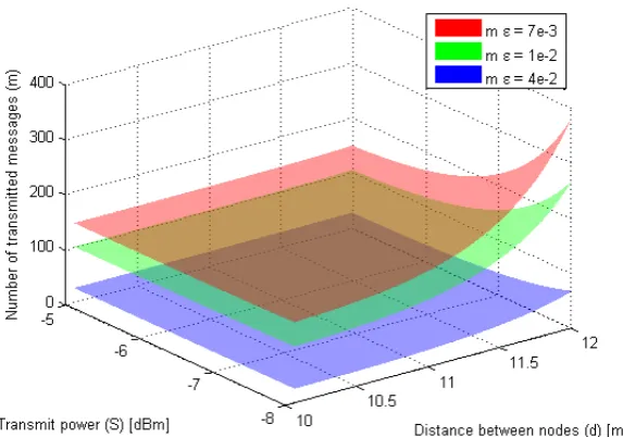
energy A S m( , , )δ with transmit power S under the in-fluence of large-scale fading for different values of the estimation quality , for a fixed distance d between transmitter and receiver nodes. Figure 2 shows the de- pendence of m with S and d under large-scale fading. It can be seen that for S fixed, as d grows, m has to be in- creased accordingly.
Since under large-scale effects the dominating factor in signal fading is the distance d between pairs, the nodes’
relative velocity is not an independent variable in the energy graphics. However, it is always possible to define a fixed
time window, e.g. ∆ =t 1s, substitute d with its defini-tion in (20), and analyze the variadefini-tion of the energy mi-nima as dictated by (24). Hence, although there is a unique relation between d and V, it is more accurate to analyze the variations the energy minima with d under this scena-rio. The figures in this section have the following simula-tion parameters:
2 4
0
,
1, 80 , 7.0146 10
/ 10, dB 1 , 3.71, 1 s
V Rx
M
S dBm K
d d ψ dB T
σ
σ γ
−
= =
=
= − ⋅
[image:5.595.152.447.233.457.2]= = = .
Figure 1. Number of transmitted messages m and Energy required A(S, m, d) as a function of transmit power S for large-scale fading, for different clock offset estimation qualities e using one-way messages.
[image:5.595.156.443.506.707.2]5. Summary and Discussions
Time synchronization for a WSN can be achieved by means of parameter estimation techniques which require a number of messages to be transmitted from a sender to a receiver node. The minimum amount of total energy required for achieving a desired estimation quality
is represented by the product of the transmit power S, num-ber of messages m and the average message delay d. By introducing the concept of outage probability of the wire-less channel for large-scale fading, a minimization prob-lem can be stated for the total energy function. The reso-lution of the entire system finds the energy-optimal work-ing point which represents a lower bound for the estima-tion quality. We have also analyzed the effect of distance and relative movement between sensor nodes and pre-sented a set of equations describing their impact on the system’s parameters, which constitutes an interesting and realistic problem to real-world applications. The general results obtained in this work have been applied to the particular case of Gaussian perturbations for the Cramer- Rao efficient, unbiased offset estimator ˆθ. For other estimators that do not fulfill these conditions, the estima-tion error σθ2ˆ shall be used instead of the FisherInfor-mation function in order to compute the theoretical limits for that particular case. As part of our future work, we are working on the small-scale effects counterpart when moving targets are synchronizing in a WSN.
Finally, unlike under large-scale effects where the dis- tance between nodes plays a predominant role in the ener- gy minimization problem, under small-scale effects the relative velocity between nodes is a determining factor in the synchronization accuracy, due to the Doppler spread effect [19]. Thus, our aim is to complete a comprehen-sive analysis of “energy-synchronization quality” trade- off under both fading scenarios as part of our future work.
REFERENCES
[1] A. Swami, Q. Zhao, Y. Hong and L. Tong, “Wireless Sensor Networks, Signal Processing and Communications Perspectives,” John Wiley & Sons, Hoboken, 2007, pp. 9-89.
[2] F. Ren, C. Lin and F. Liu, “Self-Correcting Time Syn-chronization Using Reference Broadcast in Wireless Sensor Network,” IEEE Wireless Communications, 2008.
[3] L. Schenato and G. Gamba, “A Distributed Consensus PROTOCOL for Clock Synchronization in Wireless Sensor network,” Proceedings of the 46th IEEE Confe-rence on Decision and Control, New Orleans, 2007.
[4] T. Locher, P. Von Rickenbach and R. Wattenhofer, “Sensor Networks Continue to Puzzle: Selected Open Problems,” Proceedings of the 9th International Confe-rence on Distributed Computing and Networking, 2008.
[5] P. Briff, F. Vargas, A. Lutenberg and L. Rey Vega, “On
the Trade-Off of Power Consumption and Time Synchro-nization Quality in Wireless Sensor Networks,” Proceed-ings of the 11th IEEE Conference on Sensors, Taipei, 2012, pp. 1927-1930.
[6] J. Elson, L. Girod and D. Estrin, “Fine-Grained Network Time Synchronization Using Reference Broadcasts,” Proceedings of the 5th Symposium on Operating Systems Design and Implementation, Boston, 2002.
[7] S. Ganeriwal, R. Kumar and M. Srivastava, “Timing- Sync Protocol for Sensor Networks,” SenSys ’03, Los Angeles, 2003.
[8] K. Noh, E. Serpedin and K. Qaraqe, “A New Approach for Time Synchronization in Wireless Sensor Networks: Pairwise Broadcast Synchronization,” IEEE Transactions on Wireless Communications, Vol. 7, No. 9, 2008.
[9] E. Serpedin and Q. Chaudhari, “Synchronization in Wire- less Sensor Networks: Parameter Estimation, Perfor- mance Benchmarks, and Protocols,” Cambridge Univer-sity Press, Cambridge, 2009.
[10] Q. Chaudhari, E. Serpedin and K. Qaraqe, “Cramer-Rao Lower Bound for the Clock Offset of Silent Nodes Syn-chronizing through a General Sender-Receiver Protocol in Wireless Sensornets,” 16th European Signal Processing Conference (EUSIPCO), Lausanne, 2008.
[11] F. Ferrari, M. Zimmerling, L. Thiele and O. Saukh, “Effi- cient Network Flooding and Time Synchronization with Glossy,” IEEE 10th International Conference on Infor- mation Processing in Sensor Networks (IPSN), 2011, pp. 73-84.
[12] G. Deng and F. Zhang, “A Power Management for Prob-abilistic Clock Synchronization in Wireless Sensor Net-works,” IEEE International Conference on Communica-tion Technology, 2006, pp. 1-4.
[13] T. Schmid, P. Dutta, and M. B. Srivastava, “High-Reso- lution, Low-Power Time Synchronization an Oxymoron No More,” Proceedings of the 9th ACM/IEEE Interna- tional Conference on Information Processing in Sensor Networks, 2010, pp. 151-161.
[14] M. Akhlaq and T. R. Sheltami, “Rtsp: An Accurate and Energy-Efficient Protocol for Clock Synchronization in Wsns,” 2013.
[15] M. Maroti, B. Kusy, G. Simon and A. Ledeczi, “The Flooding Time Synchronization Protocol,” Proceedings of 2nd International Conference on Embedded Networked Sensor Systems, 2004, pp. 39-49.
[16] A. Goldsmith, “Wireless Communications,” Cambridge University Press, Cambridge, 2005, pp. 24-179.
[17] S. Kay, “Fundamentals of Statistical Signal Processing,” Prentice Hall, Upper Saddle River, 1993, pp. 27-77.
[18] Texas Instruments Inc., “Cc2520 Data Sheet 2.4 ghz ieee 802.15.4/zigbee rf Transceiver,” 2007.
[19] B. Sklar, “Rayleigh Fading Channels in Mobile Digital Communication Systems—Part 1: Characterization,” IEEE Communications Magazine, 1997, pp. 136-146.