Munich Personal RePEc Archive
Macroeconomic Risks and
Characteristic-Based Factor Models
Aretz, Kevin and Bartram, Söhnke M. and Pope, Peter F.
Manchester University, Warwick University, City University London
2010
Online at
https://mpra.ub.uni-muenchen.de/47344/
Macroeconomic Risks and Characteristic-Based Factor
Models
Kevin Aretz S¨ohnke M. Bartram Peter F. Pope∗
Abstract
We show that book-to-market, size, and momentum capture cross-sectional variation in ex-posures to a broad set of macroeconomic factors identified in the prior literature as potentially important for pricing equities. The factors considered include innovations in economic growth ex-pectations, inflation, the aggregate survival probability, the term structure of interest rates, and the exchange rate. Factor mimicking portfolios constructed on the basis of book-to-market, size, and momentum therefore serve as proxy composite macroeconomic risk factors. Conditional and unconditional cross-sectional asset pricing tests indicate that most of the macroeconomic factors are priced. The performance of an asset pricing model based on the macroeconomic factors is com-parable to the performance of the Fama and French (1992, 1993) model. However, the momentum factor is found to contain incremental information for asset pricing.
Keywords Fama and French model, Carhart model, asset pricing, book-to-market, size, momentum, macroeconomic pricing factors
JEL Classification G11, G12, G15
This version September 1, 2009
∗The authors are at Lancaster University Management School. Thanks are due to Michael Brennan, John Campbell,
Macroeconomic Risks and Characteristic-Based Factor
Models
Abstract
We show that book-to-market, size, and momentum capture cross-sectional variation in ex-posures to a broad set of macroeconomic factors identified in the prior literature as potentially important for pricing equities. The factors considered include innovations in economic growth ex-pectations, inflation, the aggregate survival probability, the term structure of interest rates, and the exchange rate. Factor mimicking portfolios constructed on the basis of book-to-market, size, and momentum therefore serve as proxy composite macroeconomic risk factors. Conditional and unconditional cross-sectional asset pricing tests indicate that most of the macroeconomic factors are priced. The performance of an asset pricing model based on the macroeconomic factors is com-parable to the performance of the Fama and French (1992, 1993) model. However, the momentum factor is found to contain incremental information for asset pricing.
Keywords Fama and French model, Carhart model, asset pricing, book-to-market, size, momentum, macroeconomic pricing factors
JEL Classification G11, G12, G15
1
Introduction
We offer a comprehensive multivariate analysis of the relations between shocks to macroeconomic
fundamentals suggested by prior research to be important for equity pricing and the benchmark risk
factors proposed by Fama and French (1993) and Carhart (1997). Although some of these relations
have already been considered elsewhere, e.g., evidence suggests that the Fama and French (FF)
bench-mark factors, HML and SMB, capture shocks to economic growth expectations (Vassalou, 2003; Liew
and Vassalou, 2000), default risk (Hahn and Lee, 2006; Petkova, 2006; Vassalou and Xing, 2004) and
the term structure (Hahn and Lee, 2006; Petkova, 2006), the focus of these studies is on one single
macroeconomic fundamental or on a narrow set of them. Still, as most macroeconomic fundamentals
at least partially reflect the state of the economy, they are often highly correlated, opening up the
possibility that the relations found in existing studies suffer from an omitted variables bias. As an
example, a downward revision in economic growth expectations often coincides with increasing
aggre-gate default risk due to more conservative consumer behavior and decreasing interest rates to revive
the economy. In this situation, an analysis of the univariate relation between HML or SMB and one of
these macroeconomic fundamentals can offer little insights on whether the benchmark factor captures
economic growth risk, default risk or interest rate risk.
We contribute to the existing literature in the following ways. First, we explore the links between
the macroeconomic fundamentals through a correlation analysis and Granger causality tests. We then
estimate a comprehensive macroeconomic factor (MF) model which can take account of associations
between the macroeconomic fundamentals. In this way, we are able to distinguish between the true
determinants of the benchmark factors and factors which only appear important in more narrow
settings due to their ability to proxy for the omitted true determinants. As a second contribution, we
expand the set of benchmark factors by investigating the Carhart (C) momentum factor, which is often
denoted by WML. We are aware of only a limited number of other studies testing the relation between
momentum and macroeconomic fundamentals, and these studies normally fail to find any significant
associations.1 We also expand the set of macroeconomic fundamentals by adding unexpected inflation
1More specifically, although Chordia and Shivakumar (2002) show that macroeconomic fundamentals can explain
and changes in a trade-weighted U.S. dollar exchange rate index. Although prior studies indicate that
these factors both associate with equity returns (e.g., Doidge et al., 2006; Vassalou, 2000; Chen et al.,
1986), their roles in explaining SMB, HML and WML have not been studied so far. Finally, we add the
market return as a pricing factor in our MF model. In an ICAPM world, this factor rewards investors
for bearing risks unrelated to the macroeconomic fundamentals. Still, as the market return is highly
correlated with the macroeconomic fundamentals, its inclusion would distort the links between the
macroeconomic fundamentals and the stock-based characteristics. To isolate the variation in market
returns not attributable to the macroeconomic fundamentals, we follow the recommendation of Connor
et al. (2006) and Fama (1998, 1996) and orthogonalize the market return with respect to our other
macroeconomic fundamentals.
Consistent with our intuition, we find strong evidence that macroeconomic fundamentals are
sub-stantially related. As a direct result of these relations, our analysis of the links between the benchmark
risk factors and the macroeconomic fundamentals can in some cases significantly contradict the main
conclusions of other studies. In a nutshell, our analysis corroborates the findings of other studies that
book-to-market (BM), and therefore HML, captures information about shocks to economic growth
expectations and the slope of the term structure, while size, and therefore SMB, captures information
about shocks to aggregate default risk (e.g., Hahn and Lee, 2006; Petkova, 2006; Vassalou, 2003).
Still, in contrast to other studies, we also show that SMB relates to shocks to the average level of the
term structure. Importantly, some significant associations documented in the prior literature either
change sign, e.g., the relation between HML and shocks to economic growth expectations, or become
insignificant, e.g., the relation between HML and shocks to aggregate default risk. Additional tests
show that these inconsistencies are driven by the omission of correlated factors in prior studies. We
also report findings entirely new to the literature. In particular, we find that WML captures default
risk, term structure risk, and more weakly foreign exchange rate risk.
The close relation between the macroeconomic fundamentals and the benchmark risk factors
im-plies that macroeconomic exposures should be able to approximate the exposures to the benchmark
risk factors in empirical asset pricing tests. As the benchmark risk factor exposures command strongly
significant risk premia and perform well in pricing the cross-section of most characteristic-sorted
for the MF model. To test these conjectures, we compare the relative and incremental pricing ability
of the MF model with those of models based on the market return and the FF benchmark risk factors
(the FF model) and the market return and the FF and C benchmark risk factors (the C model). We
also estimate the risk premia of the pricing factors of the individual asset pricing models. Overall, our
test outcomes indicate that shocks to economic growth expectations, aggregate default risk, the term
structure, and the exchange rate are priced. The significant risk premium on exposure to aggregate
default risk contrasts with the evidence reported in Hahn and Lee (2006) and Petkova (2006), who
find an insignificant default risk premium. We conjecture that this inconsistency might be due to the
proxy variable chosen for shocks to aggregate default risk. Our proxy variable is derived from Merton’s
(1974) contingent claims analysis (see Vassalou and Xing, 2004).
Our empirical findings further reveal that the MF model and the FF model exhibit a similar pricing
performance on 25 two-way sorted BM and size portfolios, while that of the C model is somewhat
higher. Consistent with this, the macroeconomic fundamentals render the risk premia on HML, SMB
and WML insignificant on these test assets. When our test assets are instead 64 portfolios three-way
sorted on BM, size and momentum, only the C model can correctly price the test assets, with the
MF model still achieving a markedly better pricing ability than the FF model. All three asset pricing
models perform adequately well in pricing 32 managed portfolios, i.e., eight three-way sorted size,
BM and momentum portfolios interacted with lagged macroeconomic instruments. For the three-way
sorted portfolios, the macroeconomic fundamentals are never able to drive out the significant risk
premia on either HML and SMB or HML, SMB and WML.
We interpret our results as showing that the FF benchmark factors contain important
informa-tion on macroeconomic fundamentals. The macroeconomic fundamentals could matter to investors,
either because they capture common variation in equity returns, as in the APT (e.g., Connor and
Korajczyk, 1995; Ross, 1976), or because they represent hedgeable sources of state variable risk, as
in the ICAPM (e.g., Brennan et al., 2004; Campbell, 1993; Merton, 1973). Since the macroeconomic
fundamentals explain a substantial proportion of equity return variation, but also forecast current
and future consumption (Chen, 1991), these interpretations are not mutually exclusive. On the other
hand, the pricing ability of the C model is only partially explained by our chosen macroeconomic
model that could help to explain the role of WML in pricing. As characteristic-sorted factors probably
capture macroeconomic pricing information efficiently, our results provide a justification for the usage
of characteristic-based pricing models like the FF model or the C model.
Our paper is organized as follows. In Section 2, we review the literature and provide the motivation
for our research. Research design and data are described in Section 3, which also contains the analysis
of the links between our macroeconomic fundamentals. We report our outcomes from the estimation of
risk exposures, risk premia and model specification tests in Section 4. In Section 5, we document that
our findings are largely robust to our choice of macroeconomic proxy variables. Section 6 concludes.
We offer more information on estimation methods and test assets in Appendix A and B, respectively.
2
Prior Literature
The ability of macroeconomic fundamentals to explain both equity returns and prices has been known
for some time, e.g., see the studies of Chen et al. (1986) and Chan et al. (1985). However, only after the
seminal studies of Fama and French (1993, 1992), which show that factors based on stock characteristics
like size or BM can also capture variation in equity prices, has academic research started to explore
the theoretical and empirical links between stock characteristics and macroeconomic fundamentals.
Our analysis contributes to this growing literature. In Table 1, we summarize the main findings from
studies documenting links between the FF and C benchmark factors and macroeconomic fundamentals,
including shocks to GDP (or alternatively industrial production) growth expectations, inflation, the
term structure of interest rates, the aggregate default (or survival) probability and the dividend yield.
Overall, the following conclusions can be distilled from this literature:
1. The evidence reported in Liew and Vassalou (2000) suggests that economic growth over the
subsequent year can be forecasted using HML and SMB. Kelly (2004) reports weaker evidence
that SMB can also be used to forecast future inflation. Related studies show that economic
growth risk is weakly priced at the 90% confidence level (Vassalou, 2003).
2. The evidence from asset pricing studies suggests that betas on changes in the slope of the
term structure are negative, and their magnitude decreases with BM (i.e., low BM stocks have
notion that growth stocks are higher duration assets. In cross-sectional tests, term structure risk
commands a significant risk premium (Hahn and Lee, 2006; Petkova, 2006). Similarly, betas on
changes in the aggregate default probability are negative, and their magnitude decreases with
size. Still, default risk never attracts a significant risk premium (Hahn and Lee, 2006; Petkova,
2006; He and Ng, 1994; Chan et al., 1985). Prior studies have so far not identified macroeconomic
fundamentals able to explain variation in WML (Griffin et al., 2003).
A potential difficulty in interpreting the body of literature summarized in Table 1 arises because
macroeconomic fundamentals are likely to be substantially correlated. A notable feature of the table
is that the cited studies focus on only partially overlapping sets of macroeconomic fundamentals. For
example, no prior study considers economic growth and inflation risks together with term structure
and default risks. As a result, we cannot rule out that in existing studies one macroeconomic factor
proxies for another “more fundamental” factor. There is also the possibility that beta estimates in
existing studies are biased due to correlated relevant pricing factors being omitted from an asset
pricing model. We explicitly address these concerns by estimating an MF model that includes a broad
set of macroeconomic fundamentals considered in the prior literature. We also expand the set of
macroeconomic fundamentals to include unexpected inflation (not shocks to inflation expectations, as,
e.g., used in the study of Kelly (2004)) and shocks to a U.S. composite exchange rate. Prior evidence
indicates that both factors are related to equity returns (see, e.g., Doidge et al., 2006; Vassalou, 2000;
Jorion, 1991). We also add the orthogonalized market return, because in an ICAPM world this factor
rewards investors for bearing risk unrelated to the state variables (Fama, 1996, p.460).
3
Research Design
3.1 Methodology
We now review the empirical methods used to assess (1) the time-series associations between the
macroeconomic fundamentals and the firm characteristics, and (2) the cross-sectional pricing ability
model from the following time-series regression:
Rtp−1,t =β0p+β1pRMt−1,t+β2pSM Bt−1,t+β3pHM Lt−1,t(+βp4W M Lt−1,t) +εpt−1,t, (1)
whereRpt−1,tis test portfoliop’s excess return (net return minus risk-free return),RMt−1,tis the excess
return on a value-weighted stock market index, SM Bt−1,t is the return of a portfolio long on small
and short on big market capitalization stocks (keeping BM and momentum constant), HM Lt−1,t is
the return on a portfolio long on high and short on low BM ratio stocks (keeping size and momentum
constant), andW M Lt−1,tis the return on a portfolio long on winner and short on loser stocks (keeping
size and BM constant). If we impose the restriction β4p = 0, the model shown in equation [1] is the
FF model. Otherwise, the model shown in equation [1] is the C model.
The beta coefficients of the MF model can be estimated from the following time-series regression:
Rpt−1,t=βp0+β1pM Y Pt,t+12+β2pU It−1,t+β3pDSVt−1,t+β4pAT St−1,t (2)
+β5pST St−1,t+β6pF Xt−1,t+εpt−1,t,
where M Y Pt,t+12 is the change in one-year ahead industrial production growth expectations,U It−1,t
is unexpected inflation, DSVt−1,t is the change in the aggregate survival probability, AT St−1,t and
ST St−1,t are changes in, respectively, the average level and the slope of the term structure, and
F Xt−1,t is the change in a multilateral U.S. dollar exchange rate. As discussed, this model nests all
the main macroeconomic factor models shown in Table 1, but it also includes two neglected
macroe-conomic fundamentals, i.e., unexpected inflation and shocks to the exchange rate. We also consider
an augmented version of the MF model (the AMF model) which includes the market return.
Re-sults reported in Section 4 show that around 74.2% of the variance in market returns is explained by
the macroeconomic fundamentals. Since the market return cannot be treated as exogenous, we first
orthogonalize market returns with respect to the other macroeconomic fundamentals.
We use the stochastic discount factor/generalized method of moments (GMM) methodology
pro-posed by Cochrane (2001) (1) to assess whether the macroeconomic fundamentals command significant
risk premia and (2) to evaluate the pricing ability of the models. Jagannathan and Wang (2002) show
models. When analyzing excess returns, the stochastic discount factor representation is:
0 =ppt =Et(mt+1Rpt,t+1), (3)
where ppt is the market price of portfolio p (zero for excess returns),Et(.) is the expectation operator
conditional on timetinformation,mt+1 is the linear stochastic discount factor, i.e.,mt+1 = 1−b′ft+1,
where ft+1 are the models’ pricing factors, andRpt,t+1 is portfolio p’s excess return. When examining
excess returns, the average level of the stochastic discount factor is not identified. To circumvent this
problem, we choose to set the constant to unity. We can rearrange equation [3] to obtain risk premia,
whose significance levels can be inferred with the delta method (see Appendix A).
3.2 Test Assets
We use firm characteristic-sorted portfolios as test assets throughout this study, with the firm
char-acteristics being BM, size and momentum. Moreover, we employ both unconditional and conditional
portfolios, where the conditional portfolios are interacted with lagged macroeconomic instruments. We
create one-way sorted characteristic portfolios analogous to Fama and French (1993). In particular,
we observe the BM decile breakpoints in December of yeart−1 and the size decile breakpoints and the
prior eleven month compounded return (momentum) breakpoints in June of yeart. The construction
of the momentum characteristic follows Carhart (1997). Consistent with other studies, we only use
NYSE firms to obtain the breakpoints. After identification of the breakpoints, we form value-weighted
portfolios comprising all stocks from the NYSE, AMEX and NASDAQ within each relevant range of
the sorting variable in July of year t. Portfolio composition remains fixed until June of year t+1, at
which point we reform portfolios according to the same algorithm.2
We construct two-way and three-way independently-sorted portfolios from subsets of the same
breakpoints. To limit the number of test assets, we assign firms to (1) eight (2x2x2) portfolios based
on the median breakpoints, (2) 27 (3x3x3) portfolios based on the bottom 30%, middle 40% and top
30% breakpoints, and (3) 64 (4x4x4) portfolios based on the bottom 20%, lower-middle 30%,
top-2Studies in the momentum literature, as, e.g., Jegadeesh and Titman (1993, 2001), often examine various portfolio
middle 30% and top 20% breakpoints. Similar to Liew and Vassalou (2000), we create the three-way
independently-sorted benchmark factors, i.e., HML, SMB, and WML, from the (3x3x3) benchmark
portfolios (see Appendix B for more details).
3.3 Macroeconomic Fundamentals
We now introduce the variables we use in our tests to proxy for the macroeconomic fundamentals in the
MF model. Our first macroeconomic fundamental, which is changes in economic growth expectations,
should capture revisions in investors’ cash flow (dividend) expectations. To facilitate monthly data
analysis, we select industrial production growth as our measure of economic growth rather than GDP,
which is only observable on a quarterly basis. Petkova and Zhang (2005) argue thatrealized industrial
production growth is a poor proxy for the change in economic growth expectations and its usage would
result in an errors-in-variables problem. Hence, we adopt an approach initially proposed by Breeden
et al. (1989) and later refined by Lamont (2001) and Vassalou (2003), and create a mimicking portfolio
capturing changes in one-year ahead industrial production growth expectations. Portfolio weights are
obtained by regressing the log change in realized industrial production over the subsequent year on a
set of traded base assets and a set of control variables designed to capture all anticipated information
in industrial production growth and the base asset returns.
If the mimicking portfolio approach is to be powerful, the base assets must span the space of asset
returns. Besides this, theory offers little guidance on the choice of base assets, perhaps explaining the
wide range of assets used in related prior research. Since we are interested in establishing the empirical
relations between the FF and C benchmark factors (and their underlying benchmark portfolios) and
our macroeconomic fundamentals, we are careful not to include the benchmark factors in the set of base
assets. Instead, we include the market portfolio, a long-term and an intermediate-term government
bond portfolio, a high-yield corporate bond portfolio and gold. All base asset returns are in excess of
the risk-free rate, so that mimicking portfolio weights do not need to sum to unity. During two periods
in our sample period, namely the 1987 stock market crash and the Internet bubble period, market
returns are unlikely to efficiently capture news on economic growth. To control for the possibility that
slope dummies which allow the market portfolio weight to vary during these periods.3 As controls, we
use lagged instruments found in prior studies to predict variation in stock returns.4 In two alternative
specifications, we also add the one-month or one-year lagged base asset excess returns. A complete
list of the base assets and control variables is presented in the footnote of Table 2.
We follow Vassalou and Xing (2004) in using an equally-weighted average of stock-level survival
probabilities as the aggregate market estimate, where we derive a firm’s survival probability over the
subsequent year according to the contingent claims model of Merton (1974). Monthly shocks to the
aggregate survival probability are defined as changes in the original time-series. Unexpected inflation
is approximated through realized inflation minus the fitted value from an MA(1) process (Fama and
Gibbons, 1984).5 We employ two interest rate term structure risk factors: (i) the change in the average
level of the term structure (i.e., the change in the mean of the 3-month Treasury bill yield and the
10-year Treasury bond yield); and (ii) the change in the term structure slope (i.e., the change in the
difference between the 10-year Treasury bond yield and the 3-month Treasury bill yield). Finally, we
capture exchange rate risk through the change in a U.S. composite exchange rate.
3.4 Data and Sample
We obtain the data used to form the benchmark portfolios and characteristic-based factors from the
intersection of CRSP and COMPUSTAT. We exclude firms with negative book values and issues
other than common stock. Equivalent to Fama and French (1993), we define the book value as the
COMPUSTAT book value of stockholders’ equity, plus balance-sheet deferred taxes and investment
tax credits, minus the book-value of preferred stock, where the value of preferred stock is either the
redemption, liquidation, or par value (in this order). The original FF benchmark portfolios and factors
and the risk-free rate are from Kenneth French’s website. The dividend yield on the S&P500 index
is from Robert Shiller’s website. We obtain the aggregate survival probability from January 1975 to
3The exclusion of the slope dummies does not materially affect the relations between the stock characteristics and
the macroeconomic fundamentals. However, their inclusion renders the mimicking portfolio more similar to an out-of-sample rolling window estimate of it, while retaining the important advantage that we can correct standard errors for the additional uncertainty created by the generated regressor.
4See Ferson and Harvey (1991), Breen et al. (1989), Ferson (1989), Harvey (1989), Fama and French (1989, 1988),
Campbell (1987) and Keim and Stambaugh (1986).
5Unexpected inflation is therefore also a generated regressor. However, Pagan (1984) proves that, if the generated
December 1999 from Maria Vassalou’s website.6 We extend these data to December 2008 following
the approach of Vassalou and Xing (2004).7 Yield data on 3-month U.S. government Treasury bills,
10-year Treasury bonds, Aaa/Baa-rated corporate bond portfolios and the exchange rate (in foreign
currency per unit of home currency) between the U.S. dollar and a broad trade-weighted composite
currency index are from the Federal Reserve Bank’s website. Return data on the U.S. bond portfolios
and gold are from Ibbotson Associates. We obtain the seasonally-adjusted level of the U.S. industrial
production index and the consumer price index from DataStream. All our variables are at a monthly
frequency and are for the sample period from January 1975 to April 2008.8
3.5 Summary Statistics and Granger Causality Tests
In Table 2, we report the outcomes from OLS regressions used to find the base asset weights of the
mimicking portfolio on changes in economic growth expectations. As monthly industrial production
growth is measured over rolling one-year windows, we adjust t-statistics for the induced moving average
error in residuals using the Newey and West (1987) correction with the lag parameter l set equal to
eleven. Overall, the asset weights are fairly similar across the three model specifications shown in the
table. The t-statistics and exclusion tests both indicate that, of the base assets, the market portfolio,
the intermediate-term government bond portfolio and gold are most significantly related to one-year
ahead changes in the industrial production index. The weight of the market portfolio is reduced to
virtually zero during the 1987 stock market crash, but it is significantly higher during the Internet
bubble period.9 Some control variables, e.g., the risk-free rate, are also significant.
A central question is how well the mimicking portfolio reflects changes in one-year ahead economic
growth expectations. Across the three specifications, the lower-bound adjusted R2from a hypothetical
OLS regression of changes in industrial production growth expectations on the unexpected base asset
returns is at least 3.51%. Although this estimate is slightly lower than those reported in other studies,
6We thank Kenneth French, Robert Shiller, and Maria Vassalou for making these data available.
7The correlation coefficient between the monthly DSV series obtained from Maria Vassalou’s website and ours is 0.95
during the period from February 1971 to December 1999. We extend Maria Vassalou’s data from December 1999 to December 2008 through the prediction from an OLS regression of her series onto our series. The intercept and slope coefficient of this regression equal 0.002 and 0.918, respectively. Our main conclusions do not change, if we entirely use our own series in our empirical tests.
8Although most of our data extend to December 2008, we require the 12-month lead level of the industrial production
index to construct our proxy for changes in economic growth expectations.
9One explanation is that firms raised new capital during the initial rise of the stock market, which was subsequently
the low value is mainly driven by the fact that our sample period starts shortly after the oil crises
(i.e., inclusion of the oil crises would have increased the lower-bound to approximately 8%). Besides
this, our parameter estimates and significance levels are very similar to those reported elsewhere
(e.g., Vassalou, 2003; Lamont, 2001). In addition, we have also compounded the mimicking portfolio
to a bi-annual frequency and then computed its correlation coefficient with changes in industrial
production growth expectations obtained from the Livingston Surveys of Professional Forecasters over
the period from June 1975 to December 2007. For all three specifications, the correlation coefficient
is around 0.50, suggesting that our approach can capture a large fraction of changes in the survey
participants’ expectations. Our correlation estimates are conservative, as the survey data are based
on 14-month forecast horizons10and survey participants are no major equity investors. In the interests
of parsimony, we employ the second mimicking portfolio specification in the remainder of the study,
as this specification yields the highest lower-bound adjusted R2.11
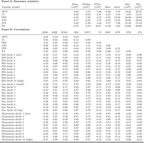
We present summary statistics on the macroeconomic fundamentals in Panel A of Table 3. The
sample mean of the mimicking portfolio on economic growth (MYP) is positive, but insignificant when
not controlling for the influence of other risk factors. Summary statistics on the benchmark portfolios
and factors are in a table in the Appendix. The most important feature of Table 3 is shown in Panel B:
several macroeconomic fundamentals are highly correlated, e.g., MYP and DSV, ATS, and STS or
ATS and STS and FX, confirming that interpretation of some prior studies could be ambiguous.
Panel B of Table 3 also shows correlations between the one-way sorted characteristic portfolios and
the benchmark risk factors and macroeconomic fundamentals. While the correlation coefficients often
suggest associations between the benchmark risk factors and the macroeconomic fundamentals, our
multivariate model results presented later will show that bivariate correlations are not always a good
guide to the sign and significance of macroeconomic exposures.
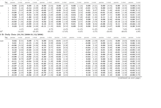
The summary statistics shown so far reveal nothing about causality between the benchmark risk
factors and the macroeconomic fundamentals. Hence, we report the outcomes from Granger causality
tests analyzing whether certain benchmark risk factors or macroeconomic fundamentals help to forecast
others in Table 4. The main idea of these tests is that, if an event causes another event, then it should
10Although survey participants are asked to predict the level of the industrial production index twelve months after
precede the other event in time. Although most of the relations between our analysis variables should
be contemporaneous, the tests in Table 4 check whether some fraction of the change in one variable
occurs before the change in another.12 In Panel A, we consider monthly data over the sample period
from January 1975 to April 2008 with the lag length set equal to one. We have checked that other lag
lengths do not substantially affect our main conclusions from these tests. Considering first the links
between the macroeconomic fundamentals, MYP and ATS seem to be exogenously determined with
respect to the other factors. However, an upward revision in economic growth expectations associates
significantly with a higher aggregate survival probability and U.S. dollar value in the future. In
a similar way, an increase in the average term structure significantly predicts a higher unexpected
inflation and U.S. dollar value and a lower aggregate survival probability and term structure slope.
In contrast, DSV and STS can be predicted by the other macroeconomic fundamentals, but cannot
predict them themselves. Both UI and FX form a feedback system with the other factors.
It is also interesting to check whether the macroeconomic fundamentals Granger-cause the
bench-mark risk factors, or vice versa. With the notable exception of UI, which will turn out to be relatively
unimportant for equity pricing, only STS can be forecasted with SMB at the 90% confidence level. In
contrast, HML can be forecasted with ATS and FX, SMB with UI and DSV and WML with MYP and
ATS. As a result, we conclude that the macroeconomic fundamentals often precede the benchmark
risk factors in time, and therefore appear more elementary. The in-sample adjusted R2s (IS-R2) are
between -0.4% (MYP) and 14.9% (FX). Finally, the low out-of-sample adjusted R2s (OOS-R2) based
on residuals constructed from estimates obtained over the prior ten years of data suggest that investors
were not able to forecast the analysis variables with any success.
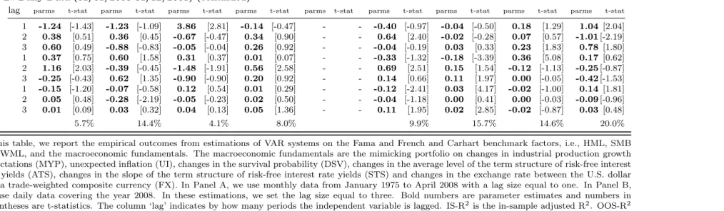
We also explore whether the causality between the macroeconomic fundamentals and the
bench-mark risk factors can change during an economic recession. To this end, we estimate the VAR system
on daily data over 2008 in Panel B. While the benchmark risk factors can be obtained at a daily
frequency from Kenneth French’s website, we construct a daily time-series for the mimicking portfolio
through combining the weights obtained from the monthly estimations in Table 2 with daily data on
the base assets. To obtain a daily estimate of the aggregate survival probability, we assume that asset
volatilities are constant over one month, and then use the Merton (1974) model to first back out daily
asset values and to then construct a firm’s default probability (see, e.g., Vassalou and Xing, 2004).
Daily time-series on the 3-month Treasury Bill yield, the 10-year Treasury bond yield and the
compos-ite exchange rate can be obtained from the webscompos-ite of the Federal Reserve Bank. Unfortunately, we
are unable to compute a daily time-series for unexpected inflation, and we therefore omit this variable
from the daily estimations. Our empirical findings reveal that the links between our analysis variables
are much stronger in an economic recession. All macroeconomic fundamentals now form a feedback
system. Next, the benchmark risk factors now often also forecast the macroeconomic fundamentals,
although they can also still be forecasted by them. Finally, the in-sample adjusted R2s (IR-R2) are
often much higher than those in Panel A, but they are always higher than those from estimations on
daily data from August 1998 to December 2008 (not reported).
4
Results
4.1 Macroeconomic Risk Exposures
We now analyze the estimation outcomes from the time-series regression in equation [2] of the one-way
or three-way sorted characteristic portfolio returns onto the macroeconomic fundamentals. We use
Hansen’s (1982) GMM methodology to estimate all parameters, with standard errors corrected for
the additional uncertainty induced through the generated regressor MYP. We offer more details on
the GMM methodology in Appendix A. We show the regression coefficients and t-statistics of the
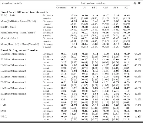
one-way sorted portfolios in Figure 1. In Panel A of Table 5, we report χ2 statistics testing whether
the spread in the macroeconomic risk exposures is significantly different from zero across the one-way
sorted characteristic portfolios. Although the table does not report adjusted R2s for the one-way
sorted portfolios, we note that these range from 49.4% to 70.4%, suggesting that the macroeconomic
fundamentals capture a large fraction of the variation in the one-way sorted portfolio returns.
In Figure 1, we illustrate that, of the macroeconomic fundamentals, MYP, DSV, and STS play
significant roles in explaining the one-way sorted characteristic portfolio returns. The absolute values
of the t-statistics on the MYP betas are greater than 2.0 on all 30 characteristic portfolios. In contrast,
their absolute values on the DSV and STS betas are only greater than 2.0 on 24 and 26 portfolios,
and negatively to STS. More importantly, the figure shows vividly that some macroeconomic exposures
strongly relate to the BM, size and momentum characteristics of the portfolios. For instance, when
we compare macroeconomic exposures across the BM deciles, the MYP exposures generally decrease,
while the DSV, STS and FX exposures increase with BM. Panel A of Table 5 reveals that the spread
in the MYP and STS exposures are strongly significant, while those in the DSV and STS exposures
are more weakly significant. The figure also illustrates that the DSV, ATS, STS, and FX exposures
almost monotonically decrease with the size characteristic of the size-sorted portfolios, while only the
smallest firm decile has a lower MYP exposure than the others. The spread in exposures is strongly
significant for MYP, DSV and ATS, and more weakly significant for STS. Finally, the DSV, STS and
FX exposures all relate to the momentum characteristic of the momentum-sorted portfolios, with all
spreads being significant at the 95% confidence level.
As the size, BM and momentum firm characteristics are themselves correlated, our evidence on the
one-way sorted portfolios is not unambiguous. More specifically, the correlation coefficients between
the BM and size decile, the BM and momentum decile and the size and momentum decile are -0.17,
0.11, and 0.17, respectively. Hence, the spread in one specific macroeconomic exposure across the size
portfolios could be driven by the fact that small (large) firms often have high (low) BM ratios. For
this reason, Fama and French (1993) orthogonalize benchmark portfolios with respect to size (BM)
when constructing the BM (size) benchmark portfolios underlying HML (SMB). We expect that the
evidence based on three-way sorted portfolios should therefore draw out more clearly the roles of each
firm characteristic in capturing macroeconomic exposures.
We report the estimation outcomes from the three-way sorted benchmark portfolios and RM,
HML, SMB, and WML in Panel B of Table 5. The t-statistics on the macroeconomic exposures of the
benchmark risk factors can be interpreted as tests of differences in macroeconomic exposures across
the top three and the bottom three BM, size or momentum deciles, respectively, after controlling for
correlation between firm characteristics. Most results in the table align with those obtained from the
one-way sorted portfolios. For example, consistent with the exposures of the benchmark portfolios,
HML loads negatively on MYP and positively on STS, SMB loads positively on DSV and ATS, and
WML loads negatively on DSV, STS and FX. Two important inconsistencies between the results on
for other firm characteristics, HML relates no longer to DSV, and SMB relates no longer to MYP. We
can explain these inconsistencies by noting that both size and momentum capture DSV risk, and that
controlling for these relations probably drives out the link between BM and DSV. In a similar way,
controlling for the relation between BM and MYP might drive out the link between SMB and MYP.
While our results on the relations between the benchmark risk factors and UI and FX and those on
the relations between WML and the macroeconomic fundamentals are entirely new to the literature,
it is instructive to compare other results in our analysis with those from the prior literature. Our
results contradict the prior literature in three main ways:
1. Liew and Vassalou (2000) and Kelly (2004) find a significantly positive relation between HML
and MYP. In contrast, we find a negative relation in Table 5. We can account for the difference
by observing that these two prior studies do not control for term structure risk. Our summary
statistics reveal that MYP has a positive correlation with ATS and STS. When we drop ATS
and STS, add RM and restrict our sample period to 1978 to 1996 (the sample period analyzed
in these studies), the relation between HML and MYP turns negative.
2. In contrast to our main findings, Hahn and Lee (2006) and Petkova (2006) obtain no evidence
that SMB associates with term structure risk. We conjecture that this difference could be driven
by correlation between ATS and STS, on the one hand, and MYP and FX, on the other. When
we end our sample period in 2001 (which is the end of their sample period; unfortunately, the
start of their sample period is before ours), include RM and drop MYP and FX, we also find an
insignificant association between SMB and ATS.
3. Vassalou and Xing (2004) find a negative relation between HML and DSV. In contrast, we find
no significant association between these two variables after controlling for other macroeconomic
fundamentals. We conjecture that the findings in Vassalou and Xing (2004) are an artifact of
the positive correlation between MYP and DSV. Dropping MYP from our MF model and ending
our sample period in 1999 (which is the end of their sample period; unfortunately, the start of
their sample period is before ours), HML loads significantly and negatively on DSV.
While our remaining results confirm those reported in the literature, the above cases confirm the
MF model includes more macroeconomic fundamentals than those in prior studies, we acknowledge
that it could also be incomplete. Our inferences are thus vulnerable to a similar critique.
4.2 Unconditional Pricing Tests
We evaluate the cross-sectional pricing ability of the MF, FF and C models in this section. If the success
of the FF and C models in pricing characteristic portfolios can be explained by the benchmark risk
factor exposures serving as proxies for macroeconomic exposures, then the macroeconomic exposures
of the MF model should at least in theory perform similarly in pricing. On the other hand, if either the
FF or C model outperforms the MF model, this indicates that the firm characteristics capture a richer
set of information on priced factors than that captured by the macroeconomic fundamentals. This
section analyzes unconditional test portfolios. In particular, we run our pricing tests on the 25 two-way
sorted BM and size portfolios that are widely used in the literature. We also consider 64 three-way
sorted BM, size and momentum portfolios, as a larger number of test assets with greater spreads in
expected returns should increase explanatory power in the presence of measurement errors endemic
in macroeconomic data, i.e., a lack of timeliness and/or predictability in revisions. We estimate all
models with the GMM to avoid a bias in standard errors (see Appendix A).
Our estimation outcomes are in Table 6, which first reports the relations between the relevant set
of pricing factors and the stochastic discount factor. Significant coefficients indicate that, conditional
on the other pricing factors of a model, a pricing factor helps to correctly price the test portfolios.
Below the loadings on the stochastic discount factor, we show the estimated risk premia, which reveal
whether each pricing factor is priced. To evaluate the pricing ability of each model, we also report
Hansen’s (1982) J-test and the adjusted R2 from an OLS regression of mean portfolio returns on
exposures. For the FF and C models, our results based on the 25 portfolios are close to those shown
on the 64 portfolios. For the MF and AMF models, we find similar parameter estimates on both sets
of test portfolios, but consistent with our expectations significance levels are lower for the smaller
set of test portfolios. As a result, we only report the estimation outcomes from the larger set of 64
portfolios. Still, it is worthwhile highlighting that the abilities of the MF and FF models to price the
25 test assets are relatively similar. For example, the adjusted R2s of the MF and the FF models are
We show our results based on the 64 test portfolios in Table 6. Several of the macroeconomic
fun-damentals capture variation in the stochastic discount factor, i.e., MYP, DSV, ATS, STS, and FX are
all highly significant at conventional levels. However, a different set of pricing factors could command
a significant risk premium, as the macroeconomic fundamentals are highly correlated (Cochrane, 2001,
pp.260-262). Notwithstanding this argumentation, we find that the same macroeconomic
fundamen-tals are priced at the 99% confidence level. Augmenting the MF model by adding the orthogonalized
market return (RM*) does turn the loading on the stochastic discount factor and the risk premium of
UI significant, while it renders the risk premium of STS insignificant. In addition, the risk premium
on DSV is now only significant at the 95% confidence level. The RM* factor obtains a significant
stochastic discount factor loading and risk premium, and its inclusion in the MF model increases the
adjusted R2 from 30.9% to 35.9%.13
The sign of the risk premia are in accordance with economic intuition. We have already shown
that high (low) BM assets often have small (large) positive MYP betas and small (large) negative STS
betas. In light of the more negative risk premium on MYP than on STS and the almost equal spread in
exposures on these macroeconomic fundamentals, MYP can help to explain the average return spread
between BM portfolios. Similarly, small (big) size assets have large (small) positive DSV betas and
small (large) negative ATS betas, with the spread in the DSV betas being much larger than that in the
ATS betas. In combination with a positive risk premium, DSV can help to explain the average return
spread in the size portfolios. Finally, high (low) momentum assets have small (large) positive DSV
betas, large (small) negative STS betas and small negative (small positive) FX betas. As a result,
the positive risk premium on DSV drives up the average return prediction of losers relative to that
of winners, while the negative risk premium on STS drives the same down to a slightly lower extent.
Hence, we conclude that the macroeconomic fundamentals seem unable to explain momentum.
Our empirical outcomes on the FF and C models are consistent with prior studies. All the FF and
C benchmark factors strongly associate with the stochastic discount factor and also obtain significant
risk premia. The significant risk premium on SMB reveals that the size effect has re-emerged over the
last years. Our evaluation statistics (i.e., the adjusted R2s and the J-tests) and Figure 2 suggest that
13As a robustness check, we also use the Fama and MacBeth (1973) methodology to compute the risk premia of the
the MF and FF models cannot correctly capture variation in the equity prices of the 64 portfolios,
with the MF model working slightly better than the FF model. The C model displays the best pricing
ability, which is not surprising given that its pricing factors include a momentum portfolio (WML).
Our empirical analysis indicates that foreign exchange rate risk can be important when pricing the
cross-section of average equity returns, as FX loads significantly on the stochastic discount factor and
also attracts a significant risk premium. In contrast, inflation risk becomes only important once we
add the orthogonalized market return to the other pricing factors. Again, we find it illuminating to
compare our asset pricing results with those obtained in the prior literature. Two major differences
should be highlighted and explained:
1. Hahn and Lee (2006) and Petkova (2006) fail to obtain a significant risk premium on changes in
aggregate default risk in their cross-sectional tests. In contrast, DSV commands a significantly
positive risk premium in our tests. The difference can be explained by noting that prior studies
use the credit spread as their proxy for default risk. In this context, the findings of Longstaff et al.
(2005) and Elton et al. (2001) are interesting, which suggest that the credit spread only partially
reflects default risk (mostly <50%). Our contingent claims analysis-based proxy appears more
powerful in reflecting changes in the aggregate default probability.
2. Petkova (2006) shows that economic growth risk, computed using a methodology similar to ours,
does not command a significant risk premium in the presence of other pricing factors. We cannot
confirm this finding. While MYP and STS exhibit a high degree of correlation and clearly carry
important common information, exposures to both macroeconomic fundamentals significantly
explain average returns and both attract significant risk premia in our analysis.
4.3 Conditional Pricing Tests
Following earlier studies, e.g., Hodrick and Zhang (2001) or Cochrane (1996), we also consider the
pricing ability of the unconditional pricing models on conditional assets, i.e., on assets with
time-varying weights equivalent to dynamic trading strategies.14 To this end, we multiply the (2x2x2)
three-way sorted portfolios by an instrument set, which contains a constant, the aggregate dividend yield,
the default yield spread, and the government bond term spread, to obtain 32 managed portfolios. In
this way, the magnitude of the long and the short positions in the eight zero investment portfolios
depends on the business cycle. More information on the definition of the instruments is offered in
the footnote of Table 7. The instruments are lagged by two periods to avoid overlap with the test
assets. We ensure that the assets’ scale is roughly equal by subtracting 0.04 from the dividend yield
and multiplying all instruments by 100 (Cochrane, 1996, p.588). Given the evidence in Lewellen et al.
(2006), it is important to compare the estimates, significance, and pricing ability of the models across
alternative test portfolios to assess the robustness of our prior outcomes.
Our estimation outcomes reported in Table 7 and shown in Figure 3 suggest that the MF model
does slightly better than the FF model and somewhat worse than the C model in pricing the 32 test
portfolios. The links between the macroeconomic fundamentals and the stochastic discount factor and
the risk premia are often close to those found on the unconditional test assets. Two notable exceptions
are that the loadings of MYP and FX on the stochastic discount factor and their risk premia are no
longer significant. The differences in significance are very likely driven by smaller spreads in average
returns on the test portfolios, and thus lower statistical power. When regarding the AMF model, RM*
again loads significantly on the stochastic discount factor and also obtains a significant risk premium.
Surprisingly, however, the sign of the RM* estimates has changed. Our estimation outcomes on the
FF and C models are almost equal to those found previously. An important difference is that, in both
models, SMB no longer commands a significant risk premium at the 95% confidence level, indicating
that the characteristic-factor models also suffer from the lower spreads in average portfolio returns.
Overall, all models seem fairly capable of correctly pricing the 32 conditional portfolios.
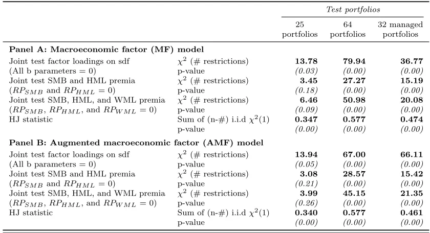
4.4 Incremental Pricing Ability of HML, SMB, and WML
Our earlier results are informative about the relative pricing performance of the three models. An
al-ternative perspective is to consider the incremental pricing ability of the FF and C benchmark factors
when added to the MF (or AMF) model. If the FF and C factors do not contain incremental
informa-tion, the macroeconomic fundamentals should drive out their significant risk premia. In Table 8, we
offer the outcomes from model specification tests and tests of incremental pricing ability. The model
funda-mentals are always jointly significant and that the Hansen-Jagannathan (HJ) distance always rejects
the MF and AMF models at conventional levels (see Hansen and Jagannathan, 1997; Jagannathan
and Wang, 1996, on computation and asymptotic distribution of the HJ distance).
Our tests of incremental pricing ability reveal that neither the benchmark factors specified by the
FF model nor those specified by the C model contain incremental information beyond our
macroe-conomic fundamentals when pricing BM and size-sorted assets. Focusing first on the unconditional
models, if we add HML and SMB or HML, SMB and WML to the macroeconomic fundamentals, the
risk premia on the FF benchmark factors or the C benchmark factors are jointly insignificant on the
25 portfolios. Our evidence hence suggests that the macroeconomic fundamentals adequately capture
risks associated with BM and size. We can draw the same conclusions when we consider the AMF
model. Further, when we analyze three-way sorted portfolio, i.e., the 64 unconditional portfolios or
the 32 conditional portfolios, then the macroeconomic fundamentals can never drive out the significant
risk premia of the FF or C benchmark factors. We conclude that HML and SMB or HML, SMB and
WML contain information not captured by the macroeconomic fundamentals which is necessary to
correctly price portfolios reflecting risks associated with BM, size and momentum.
Overall, these results strongly suggest that the success of the FF model in pricing BM and
size-sorted test assets stems from its ability to capture exposures to the macroeconomic factors included
in our MF model. In summary, the pricing ability of the MF and the FF models are comparable on
characteristic portfolios and on alternative portfolios. Also, when we use BM and size test portfolios
the macroeconomic fundamentals render the FF benchmark factors’ risk premia insignificant. At the
same time, the C model outperforms both the MF and AMF models, as well as the FF model.
5
Robustness Tests
Our analysis is complicated by the fact that proxy variables often only imprecisely measure the true
macroeconomic fundamentals explaining variation in equity returns and prices. One manifestation of
this problem is that macroeconomic proxy variables normally relate more weakly to the cross-section
of average equity returns than return-based pricing factors, as, e.g., HML, SMB and WML (see the
discussion in Cochrane, 2001). A reason for the weaker relation is that, as a result of reporting lags, it
macroeconomic data are subject to subsequent revisions, e.g., when the definition of a macroeconomic
indicator changes, implying that investors at the time perceived different shocks to the macroeconomic
fundamentals than those suggested by the revised data. Finally, macroeconomic proxy variables are
often summary measures of broader phenomena, e.g., in our study we attempt to capture the whole
term structure of interest rates through its average level and its slope. The imprecise nature of the
macroeconomic data implies that it is important to verify that our main conclusions are not driven
by our choice of proxy variables. This is the objective of this section.15
MYP:(1) We re-compute the mimicking portfolio using real-time data from the Federal Reserve
Bank of Philadelphia. The real-time data feature the realizations of the industrial production index
as experienced by market participants at the time. Our findings reveal that our previous conclusions
continue to hold, although the relations between HML and STS and between SMB and ATS are now
only significant at the 90% confidence level. (2) If the base assets’ ability to reflect news changes over
time, then our assumption of constant mimicking portfolio weights could be problematic. As a result,
we also compute MYP using recursive out-of-sample windows of initially 48 observations. Although
we are unable to adjust standard errors for the additional uncertainty induced through MYP in this
setting, our unadjusted outcomes reveal that all benchmark risk factors now reflect economic growth
risk at the 99% confidence level. In addition, HML now relates significantly to DSV and ATS and
no longer to STS, while SMB does no longer capture interest rate risk. In the cross-sectional tests,
UI now commands a significant risk premium, whereas the risk premium on STS, while still being
significant, changes its sign. Other findings are qualitatively similar.
(3) Another concern is that the mimicking portfolio simply proxies for the market portfolio, one of
its base assets. We therefore replace the market portfolio with (a) eight three-way sorted benchmark
portfolios and (b) five industry portfolios from Kenneth French’s website. The factor loadings on HML
are -1.55 (t-statistic of -1.19)16 and -1.98 (t-statistic of -2.35), respectively. In both cases, the MYP
risk premium is significant at the 90% confidence level (t-statistics of -1.87 and -2.13, respectively).
Other findings remain unaffected, except that HML no longer relates to STS and the FX risk premium
15We thank our referee for motivating this analysis. Note that we only shortly summarize the main findings from our
robustness checks in this section. A more detailed description including tables can be obtained upon request.
16When we include the three-way sorted benchmark risk factors in the mimicking portfolio, the moments from the
is no longer significant in the first case.17 (4) As a further check, if MYP simply proxies for the market
portfolio, we should be able to replace it with the market portfolio and still find similar results. Our
evidence reveals that the spread in the market portfolio exposures across the BM deciles is, at best,
weak (from 1.18 to 0.83). In combination with an estimated market risk premium of 0.80%, the market
portfolioreduces the expected return prediction on a BM spread portfolio (BM10-BM1) by 0.22%. As
MYP increases this prediction by 0.47%, these pricing factors cannot be equivalent.
UI:We also construct UI from recursive out-of-sample windows of initially ten years. As the
cor-relation coefficient between our in-sample and our out-of-sample estimate of UI equals approximately
0.95, none of our main findings were substantially affected.
DSV:Although our proxy variable derived from Merton’s (1974) contingent claim analysis should
reflect changes in aggregate default risk more accurately than others based on bond data (see Elton
et al., 2001), we also check whether our main outcomes continue to hold under these alternative proxy
variables. To this end, we first replace DSV with the return spread between a high-yield corporate
bond portfolio and a long-term government bond portfolio. In this case, the new default risk proxy
still associates positively and significantly with SMB, but not with WML. We also find that the slope
coefficients of the interest rate variables become less significant, with, however, only ATS turning
insignificant. The lower significance levels can be explained by the fact that the new default risk proxy
also captures interest rate risk (i.e., its correlation coefficients with ATS and STS are 0.50 and 0.26,
respectively). The link between WML and FX disappears, too. Although risk premia estimates are
similar to before, they show lower significance levels, i.e., only MYP, ATS and surprisingly UI are now
significant. In contrast, when we proxy for changes in aggregate default risk through the change in the
yield spread between a high-yield corporate bond portfolio and a long-term government bond portfolio
(which should relate negatively to DSV), then our outcomes align far more closely with those in the
tables. Two important differences are that SMB now relates significantly to STS (and not to ATS)
and that UI attracts a significant risk premium in the cross-sectional tests.
ATS and STS:Most other studies use one and not two proxy variables to capture news on the
term structure. As a result, we investigate whether it is important to approximate the term structure
17The missing link between HML and STS can be explained by the fact that assets with a high interest rate sensitivity
through both its average level and through its slope by including either ATS or STS in our tests. Our
outcomes reveal that HML and WML only reflect changes in the slope of the term structure (STS), i.e.,
the absence of STS fails to render the loading of ATS on HML or WML significant. In contrast, SMB
only captures changes in the average level of the term structure (ATS). Other time-series relations,
risk premia and significance levels are close to those shown before.
FX:(1) We first replace the nominal version of the broad foreign exchange rate index with its real
(i.e., inflation-adjusted) version. This does not change any of our main conclusions. (2) We also split
the broad index into one capturing exchange rates with respect to major trading partners and one
capturing exchange rates with respect to minor trading partners. The main idea is that, in theory, an
international pricing model should include exchange rates with respect to all other countries. However,
the exchange rates with respect to major trading partners should be more important than those with
respect to minor trading partners. Our findings show that WML only reflects foreign exchange rate
risk with respect to major trading partners at the 95% confidence level. Other factor loadings and
their significance levels remain close to before. In the cross-sectional pricing tests, however, we find
that both FX indexes command a significant positive risk premium, with other risk premia not being
greatly altered. (3) Finally, as only FX can be forecasted with a positive adjusted R2 in the
out-of-sample VAR tests, we replace it with the residual from an ARIMA(1,0,1). In this case, both HML
and SMB suddenly reflect exchange rate risk, while the loading of FX on WML turns insignificant.
Further, the slope coefficient of UI on HML and SMB is now significant at the 90% confidence level.
In the cross-sectional tests, the risk premium on FX is now very close to zero.
Overall, our main conclusions seem largely robust with respect to our choice of macroeconomic
proxy variables. Next, even if one of our main findings changes, we can often explain the inconsistency
through an undesirable feature of the alternative proxy variable. However, we agree that our robustness
checks only consider alternative proxy variables, and not necessarily efficient measures of the true
macroeconomic fundamentals. As a result, one cannot completely rule out that the relations between
the benchmark risk factors and the true macroeconomic fundamentals could be different from those
6
Conclusion
Several recent studies illustrate that the success of the Fama and French (1997, 1996) model in pricing
characteristic-sorted portfolios is attributable to its ability to capture information on macroeconomic
risk factors. However, as most of these studies analyze one macroeconomic fundamental or at best
a narrow set of them (e.g., see Hahn and Lee, 2006; Petkova, 2006; Vassalou and Xing, 2004;
Vassa-lou, 2003), their empirical findings are not completely unambiguous. We contribute to this literature
through a multivariate analysis based on a more comprehensive set of macroeconomic fundamentals.
Our model controls for correlation between macroeconomic fundamentals considered in the prior
lit-erature, and it adds to them unexpected inflation and shocks to a compound U.S. dollar exchange
rate. Further, we examine for the first time the relation between the momentum-based factor WML
(see Carhart, 1997) and macroeconomic fundamentals. Finally, we follow the advise of Connor et al.
(2006) and Fama (1998, 1996) and deal with the confounding impact of the market return on the other
pricing factors by orthogonalized it with respect to the macroeconomic fundamentals.
Our analysis reveals that macroeconomic fundamentals exhibit strong contemporaneous links, and
that changes in economic growth expectations and the term structure Granger-cause several of the
other macroeconomic fundamentals. We also show that the macroeconomic fundamentals seem more
elementary than the benchmark risk factor. Next, our empirical tests confirm much of the evidence
reported in prior studies. For example, we show that BM conveys useful information about term
structure risk, and size about default risk. However, we also obtain results that directly contradict
prior research. Specifically, BM does not proxy for default risk exposure after controlling for term
structure risk. Furthermore, BM reflects exposure to economic growth risk with the opposite sign to
that reported in the prior literature. Similarly, size conveys information about term structure risk.
We also report results entirely new to the literature. For example, we find that WML is significantly
associated with default, term structure and foreign exchange rate risks.
In various cross-sectional pricing tests, we first document that the majority of the macroeconomic
fundamentals command significant risk premia. More importantly, we find that, on three-way sorted
BM, size, and momentum portfolios, the MF model can compete with the FF model in terms of pricing
ability, but not with the C model. The pricing performance of the models is more similar when we
portfolios, the macroeconomic fundamentals render the risk premia on the FF benchmark factors and
the C benchmark factors insignificant. In contrast, they cannot render the risk premia on either set of
benchmark factors insignificant when we run our tests on three-way sorted BM, size and momentum
portfolios. As a result, the ability of the C model to price momentum-sorted portfolios cannot be
explained by the macroeconomic fundamentals considered in our study.
Ultimately, our results suggest that style-based equity investment strategies are associated with
dif-ferent macroeconomic exposures. This has potentially important implications for long-term investors,
e.g., pension funds, seeking to hedge liabilities with macroeconomic exposures through the equities
markets. As an investor’s liabilities depend on macroeconomic factors, such as the term structure,
economic growth, inflation, and the exchange rate, our results suggest that style investing can have a
References
Breeden, D. T., Gibbons, M. R., Litzenberger, R. H., 1989. Empirical tests of the consumption-based
CAPM. Journal of Finance 44 (2), 231–263.
Breen, W., Glosten, L. R., Jagannathan, R., 1989. Economic significance of predictable variation in
stock index returns. Journal of Finance 44, 1177–1190.
Brennan, M. J., Wang, A. W., Xia, Y., 2004. Estimation and test of a simple model of intertemporal
capital asset pricing. Journal of Finance 59 (4), 1743–1775.
Campbell, J. Y., 1987. Stock returns and the term structure. Journal of Financial Economics 18,
373–399.
Campbell, J. Y., 1993. Intertemporal asset pricing without consumption data. American Economic
Review 83 (3), 487–512.
Carhart, M. M., 1997. On persistence in mutual fund performance. Journal of Finance 52 (1), 57–82.
Chan, K. C., Chen, N. F., Hsieh, D. A., 1985. An explanatory investigation of the firm size effect.
Journal of Financial Economics 14, 451–471.
Chen, N. F., 1991. Financial investment opportunities and the macroeconomy. Journal of Finance
46 (2), 529–554.
Chen, N. F., Roll, R., Ross, S. A., 1986. Economic forces and the stock market. Journal of Business
59 (3), 383–403.
Chordia, T., Shivakumar, L., 2002. Momentum, business cycle, and time–varying expected returns.
Journal of Finance 57 (2), 985–1019.
Cochrane, J. H., 1996. A cross-sectional test of an investment-based asset pricing model. Journal of
Political Economy 104, 572–621.
Cochrane, J. H., 2001. Asset pricing. Princeton University Press, New Jersey.
Connor, G., Goldberg, L., Korajczyk, R., 2006. Portfolio risk forecasting, Notes on Chapter 6, The
Connor, G., Korajczyk, R., 1995. The arbitrage pricing theory and multifactor models of asset returns.
In: Jarrow, R., Maksimovic, V., Ziemba, W. (Eds.), Finance, Handbooks in Operations Research
and Management Science. North Holland, Amsterdam.
Cooper, M. J., Gutierrez, R. C., Hameed, A., 2004. Market states and momentum. Journal of Finance
59 (3), 1345–1365.
Doidge, C., Griffin, J. M., Williamson, R., 2006. Measuring the economic importance of exchange rate
exposure. Journal of Empirical Finance 13 (4-5), 550–576.
Elton, E. J., Gruber, M. J., Agrawal, D., Mann, C., 2001. Explaining the rate spread on corporate
bonds. Journal of Finance 56 (1), 1229–1256.
Fama, E. F., 1996. Multifactor portfolio efficiency and multifactor asset pricing. Journal of Financial
and Quantitative Studies 31 (4), 441–465.
Fama, E. F., 1998. Determining the number of priced state variables in the ICAPM. Journal of
Financial and Quantitative Studies 33 (2), 217–231.
Fama, E. F., French, K. R., 1988. Dividend yields and expected stock returns. Journal of Financial
Economics 22, 3–25.
Fama, E. F., French, K. R., 1989. Business conditions and expected stock returns. Journal of Financial
Economics 25, 23–50.
Fama, E. F., French, K. R., 1992. The cross-section of expected stock returns. Journal of Finance
47 (2), 427–465.
Fama, E. F., French, K. R., 1993. Common risk factors in the returns on stocks and bonds. Journal
of Financial Economics 33 (1), 3–56.
Fama, E. F., French, K. R., 1996. Multifactor explanations of asset pricing anomalies. Journal of
Finance 51 (1), 55–84.