A Test Program for Pseudo Random Numbers with Uniform Distribution EUR 3464

M

i««

J Sf

EUR 3464.C

i;aiîl:l·

IIWoBpiHiprn

IP

EUROPEAN ATOMIC ENERGY COMMUNITY ­ EURATOM

A TEST­PROGRAM

FOR

PSEUDO­RANDOM

NUMBERS

WITH UNIFORM DISTRIBUTION

by

G. FASSONE and S. ORTHMANN

1 9 6 7

Joint Nuclear Research Center Ispra Establishment ­ Italy

ÎPPÉ

Scientific Information Processing Center ­ CETIS

:51Ιΐ!..·:β,»}ίΐΐΐί,-ΪΛ

t«·-·«

Uk!

ï&Sti

Mr

i

KVITOU

ÄSffi!M::a

ítS

_m

m

p-t*

ii

LEGAL NOTICE

•tof

, , , f . « .; i¡;tií

tfrf

¡;wí

I

fe

ί ^ ^ ^ Η Η Ι Π Ι Α ί Ι V M I I M P ' U F ' * »■" «pf ι ■ I r* t ■ ti V * · ' t * " ΠΜΙΙ ï fl ' .Mml I #7" J ì f il tl fl · i l Il Itv I1l4f"fffl ■ ■ U l i IT 73 'γ This d o c u m e n t w a s prepared u n d e r t h e sponsorship of t h e Commission of t h e E u r o p e a n A t o m i c Energy C o m m u n i t y ( E U R A T O M ) .

N e i t h e r t h e E U R A T O M Commission, its contractors nor a n y person acting on their hehalf :

M a k e a n y warranty or representation, express or implied, „

accuracy, completeness, or usefulness of t h e information contained in this document, or t h a t t h e use of a n y information, a p p a r a t u s , method, or process disclosed in this d o c u m e n t m a y n o t infringe privately owned rights; or

li

»Uli*

A s s u m e a n y liability with respect to t h e u s e of, or for damages resulti from t h e use of a n y information, a p p a r a t u s , m e t h o d or process disclosed this d o c u m e n t .

imã

mg in

»MW

m

HM

m

i

'S M

m

at t h e price of F F 12.50 F B 125 D M 1 0 , Lit. 1560

FI. 9,

When ordering, please quote the EUR number and the title, which are

BBCrWW"

Ρ

m,

M

indicated on the cover of each report.

m

fwå

iîlfif?i|

i*;

ti.?·*

Printed h y Smeets

Brussels, M a y 1 9 6 7

Wm

mm.

This d o c u m e n t w a s reproduced on t h e basis of t h e hest available copy. iaiiii

ΜΓ,ι

Q*:λ . w m

ÏÏZ

au;

Dfcí

h­mbi

2i i

:iaejs­.ií

i l

UNIFORM DISTRIBUTION by G. FASSONE and S. O R T H M A N N European Atomic Energy_ Community - E U R A T O M

Joint Nuclear Research Center - Ispra Establishment (Italy) Scientific Information Processing Center - CET IS

Brussels, May 1967 - 80 Pages - FB 125

In this report is presented a lest program for pseudo-random sequences with uniform distribution in view of their applications to Monte-Carlo methods.

The distribution of pseudo-random sequences is studied in the (X, Y) plane and in the (X, Y, Z) space and the distribution of simple functions of η-tuples of pseudo-random numbers is compared with that predicted by probability theory.

EUR 3464.e

A TEST-PROGRAM FOR PSEUDO-RANDOM NUMBERS W I T H UNIFORM DISTRIBUTION by G. FASSONE and S. O R T H M A N N European Atomic Energy Community - EURATOM

Joint Nuclear Research Center - Ispra Establishment (Italy) Scientific Information Processing Center - CETIS

Brussels, May 1967 - 80 Pages - FB 125

In this report is presented a test program for pseudo-random sequences with uniform distribution in view of their applications to Monte-Carlo methods.

The distribution of pseudo-random sequences is studied in the (X, Y) plane and in the (X, Y, Z) space and the distribution of simple functions of η-tuples of pseudo-random numbers is compared with that predicted by probability theory

EUR 3464.e

A TEST-PROGRAM FOR PSEUDO-RANDOM NUMBERS W I T H UNIFORM DISTRIBUTION by G. FASSONE and S. O R T H M A N N European Atomic Energy Community - EURATOM

Joint Nuclear Research Center - Ispra Establishment (Italy) Scientific Information Processing Center - CET IS

Brussels, May 1967 - 80 Pages - FB 125

In this report is presented a test program for pseudo-random sequences with uniform distribution in view of their applications to Monte-Carlo methods.

The results obtained have been controlled with the a2-test and

nth Kolmogorov's test.

The results obtained have been controlled with the a2-test and

EUROPEAN ATOMIC ENERGY COMMUNITY - EURATOM

A TEST-PROGRAM FOR PSEUDO-RANDOM NUMBERS

WITH UNIFORM DISTRIBUTION

by

G. FASSONE and S. ORTHMANN

1 9 6 7

Joint Nuclear Research Center Ispra Establishment - Italy

Introduction

pag,

1.

1.1.

1.2.

1.3.

1./+.

1.5.

1.6.

1.7.

The

χ"

test

Statements of the problem

Linear uniformity test

Pairs uniformity test

Test for uniformity of triples ,

Test for uniformity of maximums

Test for uniformity of minimums

Test for uniformity of sums ...,

2.

The Kolmogorov's test

The runs tests

3.1.

3.2.

Runs up and down

Runs above and below the mean

k­

¿4..1.

I4..2.

4.3.

5.

6.

6.1.

6.2.

6.3.

6.1+.

Uniform random number generators

,

Multiplicative congruential generators ...

Mixed congruential generators

,

Combination of two congruential generators

Generator of generalized Fibonacci type ...

Program description

Note

Time

Space

Usage

Output

Appendix 1 - χ

2

table

Appendix 2 - Kolmogorov's table

Appendix 3 - Numerical results

References

1

2

2

k

5

6

6

7

7

8

10

10

10

1 2 1 2 1 3

14

15

1 7 2 1 2 1 2 1 2 2

26

66

73

75

79

SUMMARY

In this report is presented a test program for pseudo-random sequences with uniform distribution in view of their applications to Monte-Carlo methods.

The distribution of pseudo-random sequences is studied in the (X, Y) plane and in the (Χ, Y, Z ) space and the distribution of simple functions of η-tuples of pseudo-random numbers is compared with that predicted by probability theory.

The results obtained have been controlled with the az-test and

Introduction

In this report is developed a complete test series of

pseudo-random sequences in view of their applications to

"Monte-Carlo methods.

A classical test system has been studied by Kendall

-B.Smith [10,11,12] and consists of four tests: the frequency

test, the serial test, the gap test and the poker testo

Usually the gap test is replaced by a frequency test of the

length of runs.

In this paper we have retained only the frequency test

and the runs test where these are more significant in the

Monte-Carlo method applications. The frequency test involves

counting the number of pseudo-random numbers that are found

in subintervals of the range of generation (0,1).

Besides testing the randomness by the method of runs we must

compare the theoretical and the empirical distribution of up

and down runs and of above and

below the

mean

runs.

The two others have been omitted because they only give

information for binary 'digit distributions.

We have as well studied the distribution of pseudo-random

sequences in the (X,Y) plane and in the (Χ,Υ,Ζ.) space with the

frequency test. Lastly we have considered any simple functions

of η-tuples of pseudo-random numbers (maximum, minimum and sum)

to

see if their distribution is according to the distribution that

probability theory predicts.

The results obtained from several tests have been evaluated

with the χ

2

test and with Kolmogorov's test.

The considered series of tests is more restrictive than those

usually applied, therefore the information obtained is

particularly significant.

1„1. Statement of the

Problem

Let X be a random continuous variable defined in the

k-dimensional space R

k

and we suppose that X assumes values

X. belonging to a given set I C R , where

J

Η­

ν

I =

XJ

I and I have no common points.

r=1

We suppose that X has a distribution

P(S) =

PrjxC

S ¡'

(1.1.1)

where

S C I ,

and hence we shall obtain the probabilities

p

r

= P(i

r

)

(1.1.2)

Consider Ν independent trials, each of which has an

outcome X. and let f be the number of trials in which X . C I .

3

r

O r

We have

2 P

r

= 1

r=1

ν

2

f„ = Ν

r=1

r

(I0I.3)

Now f has a binomial distribution with mean

μ » Ν p

r

(1.1.h)

and variance

Let b e

-

( f . - N p . )

2

'

2

- L - "

r=1

x =

λ ^ ^ Γ "

°·

1

·

6)

it is k n o w n [2] that the "percentage" is defined b y the

following formula:

M *

2

<

x

! = -π7^

/

X tn/2

"

1 e

"

t/2

« (1.1.7)

I

J 2

n / 2

Γ(η/2) io

where η is the number of degrees of freedom and is in our case

η = ν - 1

(1.1.8)

The probability (1

· 1·7) is given in extensive tables, for

example [7]» for 1 ^ η ^ 100 with step 1. See also App.1.

We consider now a sequence of pseudo-random numbers

ξ ,ξ ,...,ξ , given by any generators, and determine the

i

¿

s

vectors

TL = C^j»··

0

»^)

Ήο

=

( ^k:+i

*

* * °

'

^2k (1°1·9)

\

=

^ ( M - l ) k + 1

,

" *

, S

k l i

)

Let X. ,Xp,... ,Χ«· i b e the values that the random variable X

assumes, we set

h

= P (

V

T

V

1 , 0

" '

T ) M

2

)

(1.1.10)

the parameters k,v,M.,Mp,N and calculate the probability

(1.1.7), that gives the confidence, with which we must accept

the pseudo-random sequence.

1.2. Linear Uniformity Test

Let I C R. be the unit interval (0,1) and let I be the

interval

(~~

>

~:)

with (r=0,1 ,2,. .., v) and putting k=1 ,

M. = Mp = J we have

Xj = FU-j)

(1.2.1)

We consider now Ρ as unit function, i.e.

Xj - t,

(1.2.2)

As well we have

Pj_ = Pi =

y

for every ^ ,

i,

¿

(1.2.3)

'1

2

i.e

0

(l.2ok)

solution of partial differential equations.

ν = 10

because it gives useful information about

distribution of the first decimal digit.

ν = 100

because it gives sufficient information about

numbers distribution.

1.3· Pairs Uniformity Test

Let I C E be the unit square of the (x,y) plane,

(θ 4 χ «i 1 , 0 * y £ 1) and let I ■ I

be the square

r

x\,,r

2

r1~l r1 r

2 ~

1

*2

J

^ χ < — - , - * ■ — S y < - *

V

V '

V

"

V

where varying r the pair (r., r

2

) is changed in conformity

with the sequence (1,1 ; 1,2;...; 1,v; 2,1;...; v,v).

Putting k=2, M. = Mp = j and Ρ unit function, we have:

X

d

= η

3

(1.3.1)

As well we have

ρ

= p. = ρ for every i., ip

(1.3.2)

x

1

x

2 v

¿

τ

This test is similar to that for pairs except that le

R

is the unit cube of the (x,y,z) space, and M. = M

2 = j , Ρ unit

function, Ν = 3*10^ , ν = 10 .

1·5· Test for Uniformity of Maximums

Let le R be the unit interval (0,1) and let I be the

₁

_{\ » /}

_r

interval

l·^­

, ^ J

with (r=0,1,..., v) and putting k=1,

M, = (j-l)m+1, M

2

= 3m+1 we have

Xd

_{= P t^M.,' ^+1'■···' ξ}

_Μ

2

^

(1.5.1)

Let

*

( 0

­L,&

( 6

<· ^ ^ J

(1.5.2)

we have

h

*[

Mw[

(

S

(i-l)m

+

l·

— ·

ξ

m

jm+1

If we consider m random variables, independent and

uniformly distributed over (0,1) X ,...,X , and let

X = Max (X.,...,X ) be, we have

1ü<m

Ί m

(1.5.3)

PrjX < k | = Pr]X

1

< k,...,X

m

< k

= Pr x

1

< k

Hence the distribution function

P(X) = X

m

Pr|X

m

< k = k

(I.5.U)

m

p

i

= p

i

=

ν

f o r e v e r y

i-i»

i

2 (1.5.6)

The test has been applied with N=1o\ ν = 100 and with

m = 2,5,10.

1.6. Test for Uniformity of Minimums

The test is similar to that for the maximums, putting

_. m

F ( £ ) = | l - Min (ξ

1

,ξ

2

,...,ξ

ϊη

) I (1.6.1)

i.e.

m

X

d

=

1 - Min (^(j-

l)m+1

»...^

dm+1

)

(1.6.2)

1.7. Test

for

Uniformity of Sums

This test is similar to that for maximums and minimums,

putting

im+1

X^ = \ ^ (mod. 1) (1.7.1)

1=( j-l)m+1

and we have

p

i

= p

i

=

ν

f o r e v e r

y i-i»

i

2

( 1 . 7 . 2 )

2. The Kolmogorov's Test

Let us suppose that the set I C R , in which is defined

k

the random variables X, is made up of ν sets Ε ,

_{r. ,}

_v

₀

_{, · *., r,}

such that

Ί ¿ κ

E

C E

.

for 1

< i

r ^ r ^ . . . , ^ , . . . , ^

r

1

,r

2

,...,j

2

...,r

k ±U1 J

1 *

J

2

E

v

t

. . . , v

M I

(2.1)

Let

=

Ρ(Β„

_

„ ) =

Pr(X c

E

w w

)

k

(2.2)

r

1

,..., r

k

r

1

,..., r

fc

^ ,..., r

fc

Consider N independent trials with outcome X . and let

P „

„ be the

number

of trials in which X . C E

V-'

r

k

¿

r

v-'

r

k

We have

Ρ

_ν,...,ν

= 1

P..

. = Ν

If in particular E_ _

„ i s the ipercube in the

r

l '

r

2

, , , , r

k

(X. ,X

2

,. ο ο ,Χ, ) space defined from

r

r

r

X

1 *

~

>

X

2

ζ

"ν" » ° ° * '

X

k * "v~

(2.3)

we have

W

'·· '

r

k

r., o.. ,r,

k

1

'

' k

ν

Putting

i

=

1 , 2 , . . . , k

we have f o r N -* oo

PrjD

>JÏÏ < \

­¥

°°

2 2

i-2 V (-1)^

1

e"

2T

>

λ

= k(X) (2.6)

η=1

The probability (2.6) is given, in extensive tables, for

example [15],

for 0,28 <S λ < 2.75 with step 0.01. See also

App.

2

3·

The

Runs Tests

3*1· Runs Up and Down

This criterion applies to the case in which the pseudo­

random numbers should be divided in two classes C., C

p

. Let

consider a sequence U , U.,...,U

k

,... we say that the number

U

k

€ C

1

if U

k

-U

k+1

< 0 and that U

k

« C

2

if U

k

~U

k+1

> 0. A run

is the set of numbers following each other and belonging to

the same class. The number of pseudo-random numbers in a run

is called its length. Let consider N pseudo-random numbers

and let f, be the runs numbers of length 1, we compare the

values f, with the theoretical values φ, . Por the case of

Ν = 1024 we have [l6]

Φ

1

Φ

2

Φ

3

\

\

=

c

=

=

=

213.4

93.

26,

5.

1«

.7

>9

,8

► 2

for h

>

5

for the class C.(up).

The same values are good for the numbers of class C

?

(down)

3.2. Runs Above and Below the Mean

Let consider a sequence U , U.,...,U,,... we say that

U

k

€ C.J if U

k

< 0.5 and that U

fc

€ C

2

if U

fc

> 0.5. We compare

the values f

1

with the theoretical values

φ-,. Por Ν = 1024

φ

ι

Φ

2

φ

3

φ

4

φ

5

%

φ

7

φ

8

Φ

9

\ =

-= =

= =

=

=

= =

128.0

64.0

32.0

16.0

8.0

4 . 0

2 . 0

1.0

0 . 5

0 . 5

for the class C. (above).

for h £ 10

4· Uniform Random Number Generators

The test program has been applied to a series of uniform

random number generators : moltiplicative and mixed congruential

generators, two combining two congruential generators, and one

alternative generator. We have considered binary and decimal

generators. Numerical results are presented in App. 3

4.1· Moltiplicative Conguential Generators

Consider the iterative process

U

k+1 = a Uk (

mod

* M

)

(¿+.I.I)

with

U

0

= b

where a, b, M are integer numbers and it is convenient to

choose M = 2 for a binary machine and M = 10

n

for a decimal

machine. Barnett [ï] has shown that for M = 2

n

, a, b odd and

a ■ 3 (mod 8) or a * 5 (mod 8) the period Ρ of the generator

is Ρ = 2

n

"

2

.

We have considered the following generators

RMTB

U

k + 1

= (2

17

+3)U

k

(mod. 2

3 3

) U

Q

= 1

RMTD

Uk + 1 = (25+3) Uk

(mod. 10i0)Uo = 1

RMTDL

U

k + 1

= 23 U

k

(mod 10

8

+1)U

Q

= 47594116

RMTDL was the first conguential generator and was proposed

by Lehmer . Its period is Ρ = 58882352.

IO·

ü

k+1 =

3 U

k

+ 1 0

(

u

k "

n

*1° )

(mod 10

ιυ

)

- L 10

1 0 k

_

where

[χ]

is the integral part of X«

(4.1.2)

4o2. Mixed Congruential Generators

Consider the iterative process

U

k+1

= a U

k

+ c

^

m o d M

^

(4.2.1)

with

U = b

o

where a, b, c, M are integer numbers and M = 2

n

for binary

machines and M = 10 for decimal machines.

Rotenberg [14J has shown that for M = 2

n

, a = 2

Γ

+ 1

with r>2 and c odd the full period Ρ = M is obtained.

Moreover in [4] it is shown that for M = 10

n

a = 10

r

+1,

c prime to 10 the full period Ρ of generator Ρ = M is obtained.

We have considered the following generators

RMB1

U

k + 1

= (2

1 2

+ 1) U

k

+1

(mod 2

3 5

)

U

Q

= 20867350019

RMB2

U

k + 1

= ( 2

7

+ 1)

U

k

+ . 7 8 8 ' 2

3 5

( m o d 2

3 5

)

U

Q

= 18575103187

>35·

R M B 3 U

k+1 = ( 2

+ 1)

u k +

1

(

m o d 2

)

U

o = °

To test RMD on a 35-bits binary machine we have considered

the following iterative process

U

k+1

= U

k

+ 1 0

° (

U

k "

η

·

1

°

8

)

+ 1

(

mod 1

°

1 0

)

where [x] is the integral part of X

4·3· Combination of Two Congruential Generators

Consider two pseudo-random generators

U

k+1

= a U

k

+ c

(

mod M

)

u

o

= b

V

k+1 =

a

'

V

k

+ c

' (

mod M

^

V = b'

_o

(4.2.2)

(4.3.1)

(4.3.2)

Let U[U.,U

2

,...,U.

Q

] be the vector whose ten components

are obtained in accordance with (4·3·1).

Let

η = [10 V

k + 1

] + 1 (4.3.3)

where [x] is the integral part of Xo

We have evidently 0 < η < 10 and we consider the nth component

in the vector Uo

Let

Sk+1 =

U

n 0*-3.U)

Lastly with the generator (4.3.1) we calculate a new component

V

We have considered the following generators

RANMX1 j

U

k+1 = (2

l 7

+3)U

k

(mod 2

3 5

) U

Q

= 1

V

k + 1

= ( 2

7 +

l ) V

k + 1

( m o d 2

3 5

) V

o

= 1

U

k+1

= ( 2 + 3 ) U

k

( m o d 2

)

U

o =

1

f

k+1 " v^

RANMX2

γ _ ^o1£■J.^^^Γ J.4 ( ™^A O 3 5

^

k+1

= (2 +l)V

k+1

+1 (mod 2-") V

0

= 2O86735OOI9

4·4» Generator of Generalized Fibonacci Type

Consider the iterative process

U

k

+

1 =

a U

k

+ U

k-1

<

m o d M

>

U

0

= b

U

1

= c

(4.4.1)

In [4] it is shown that for M = 1 0

n

, a = 10

r

+1, b = 0, c = 1,

the period is

Ρ = 1-c-m ( 3 · 2

η _ 1

, 4·5η)

(4.4.2)

Vie have considered the following generator

RPBD

U

k + 1

= (10^+1)U

k

+U

k-1

(mod 10

6

)

u„

= 0

U, = 1

o

1

■Λ/TT _ « 4ΓΆ\ (τη^Λ ΗΓ>6'

ü

k+1

s U

k

+ U

k-1

+

ΊΟ^ίυ^η.ΙΟ

4

) (mod 10°)

Lio

8 Uk

10

8

J

5· Program Description

It is possible to execute eight tests on a pseudo-random

numbers sequence. There are:

5o1. Linear Uniformity

It is called with IPTEST = 1 and NSET = 0

As well it is necessary to specify

Ν

total number of pseudo-random numbers to generate

ν

number of partial intervals

U

initial value of sequence

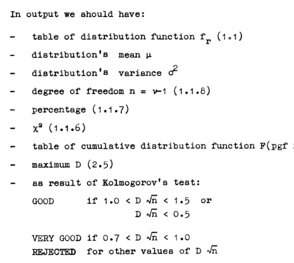
In output we should have:

table of distribution function f (1.1)

distribution's mean μ

-

distribution's variance o

degree of freedom η = v-1 (1.1.8)

percentage (1.1.7)

-

X

2

(1.1.6)

-

table of cumulative distribution function P(pgf 2)

-

maximum D (2.5)

as r e s u l t of Kolmogorov's t e s t :

GOOD

i f

1 . 0 < D Λ/ÏÏ < 1 . 5

o r

D Æ < 0 . 5

VERY GOOD if 0.7 < D Æ < 1.0

If n > 100 the program calculates the corresponding

values of χ

2

with the relation:

2

χ

2

= | ^-72x1-1 +

μ

±

because for η > 30 the χ

2

distribution is approximately normal

with mean Λ2η-1 and variance 1. Therefore the μ. values are

obtained from a table of normal distribution [5] for the values

of desired percentage.

The program calculates for the percentage 50.0 the χ

2

value, comparing it with χ

2

obtained from (1.1.6). If χ

2

< χ

2

Va' W

the program calculates a new χ

2

for probabilities greater than

50.O. If χ

2

> χ

2

is used the relation

2

χ

2

= J (Λ/2ΓΡΓ -

μ Λ

and a new χ

2

for probabilities less than 50.0 is calculated.

The considered probabilities are:

50.0, 6O.O, 70.0, 80.0, 90.0, 95.0, 97.5, 99.0, 99.5, 99.75,

99.9, 99.95

50.0, 4O.O, 30.0, 20.0, 10.0, 5.0, 2o5, 1.0, O.5, O.25, 0.1,

O.O5

The corresponding values of μ. are:

0.0, 0.253, 0.524, 0.842, 1.282, 1.645, 1.960, 2.326, 2.576,

2.807, 3.O9O, 3.291

5.2. Pairs

N

total number of

pseudo-random numbers to generate

ν

number of partial intervals for each axis (1.3)

U

initial value of sequence.

For the output the procedure is similar to that for Linear

Uniformity.

5.3. Triples

It is called with IPTEST = 3 and NSET = 0. As

well it

is

necessary to specify:

N

total number of pseudo-random numbers to generate

ν

number of partial intervals for each axis (1.4)

U

initial value of sequences

The output is similar to that for Linear Uniformity.

5·4·-6. Maximum. Minimum and.

Sum of m Numbers

These three tests being similar, have been put together.

They are called with IPTEST = 10 and NSET = 0. As well it is

necessary to specify:

Ν

total number of pseudo-random numbers to generate

ν

number of partial intervals

U

initial value of sequence

o

m «ä 10 because each m-tuple is formed with the first

m pseudo-random numbers of a vector with length 10·

5·7·-8. Runs Up and Down - Runs Above and Below the Mean

These two tests, being similar, have been put together.

They are

called

with NSET < 64 where NSET is the number of

sets. As well it is necessary to specify

Ν = 1024 total number of pseudo-random numbers to

generate for each set. Using N^1024 it is

necessary to change the theoretical values

in the main program.

U initial value of sequence.

In output we should have:

- observed average numbers of runs (up and down) with the

expected average numbers.

-

X

a

value for each set

- table of obtained runs number.

The same output is obtained in the Runs Above and Below

the Mean.

The program in the first six cases makes three successive

tests each one starting at the point where the previous test

finished.

It is necessary to specify IPTW = 0 to have the χ

2

table

in output (only for degree of freedom η < 100).

6ο Note

6.1. Time

The execution time of this program is dependent on the

total number of generated pseudo-random numbers and on the

number of partial intervals. By experience we are able to say

that to execute all the tests with the data of "Sample Input",

the program employed

~ 11,5'

for binary whether mixed or moltiplicative

conguential generators

~ 13' ■» 13,5'for decimal whether mixed or moltiplicative

generators

~ 16'

for Lehmer's generator (RMTDL)

~ 13' ■» 13,5'for binary combination of two conguential

generators

(RANMX1, RANMX2)

6o2. Space

Routine

MAIN PROGRAM

KOLM

QKHI

ARUN

ASSIN

OUT

TABLE

(TEGUS)

Locations

decimal

octal

7219

16063

266

412

3250

6262

55

67

123

173

74

112

BLOCK DATA

6.3« Usage

The program, written in FORTRAN IV for IBM 7090, requires

that the pseudo-random numbers generator has been programmed

as a FUNCTION.

The cards that eventually would have to be modified, have

an asterisk in the columns 73-80.

Cotu.

_tnn.

F o r m a t

Card A

SjJmboL

4 ­r 42,

I

M

tota? of

Q en er atea

p s e u d o

-o u /Vnbers

¡

:

­ 2o.ro :

calí

exit

M

>13 -r 34

Γ 42

h u »ni b e r ­ QL

pa r t ia E

ínter \Ta t s

K M

i^-r-36

112

start

Y a £ u e

of­

s e cjuenee

IKPV

5¥ -r 4S

tot a f

o{

S e t s l o v

t f c e

*

" ß M M S TESTS"

NSET

k9 1 5J

1 3

R

u r t i FORMI

Ta τ Esr

2 ­ P A I R S T E s r

3 ­TRiPlEs TÉST

Ί0 - ΜΛχιΜΜΜ ,

M/NlMUM AMD

S u M

O ^ ' V

n u m b e r

T E S T

1FTEST

S"-8 τ

S¿t

1 3

Tãlõl

Vtø/'

IFTEST ­ ^ O )

IP M

W o r d

Cocuwn

Format

Card d

O y moo Κ

ΐ

55 ^ 5Ύ

15

i f 3ero

t ß e s u b ­ p v ^ o

ÛLMrVi Q k H l "

\ Λ η Γ £ t Ke.

K

z

fil bfe

IFTW

t

, / ■ /

L01U.W1H

Format

Lard 2

Symboc

3

- Y 5

UAG

Ti i P. of tL

test

T/ÍLE

Worc¿

Lo Cu m n

Format

tard

¡0000

<\0

2 0 8 6 ? 5 5 θ Ο Η θ

λ

ή

UNIFORMITI TEST

T-OR

THE

FUNCTION RW6'I (iNPv) NU = AO

\0OO0 k 10%

6?

Ò500j<3 { i

UNI

FORDIT

)j

TEST

FoR. VHE FUNCTION Rf^ñ-i (iNPv) NU-

ή.

50OOO -jo

à 0 8 6 ? á 5 o o ^ g

5

-/

P A I R S

T E S T

FOR

THE

FUNCTION

RM8'I(I NPV)

ÒQOQo

Ao %02>b\i5Oojg

3

A

TRIPLES

TEST Foe

f HE

FUNCTION RM8J (l NPv)

I0OOOO

100 208é>?^SOO­/9

λΟ

10

4

MAX I MUMj Ml Ν IMUM

y

S U M TESTS

¥Od

ΤΗΈ. FUNCTION RMS A ( I NPv)

M= -JO

Ì0OOOO

-J 0 0

10 %(,%%$ 00

Ί9

ΊΟ 5 }

MAX I MUM

1

Ml NI MUM

r

5 U ^ TESTS FO(2 THE

FUNCTION

RMß-i (l NPv)

M= f

ΊΟοοοο Hoo

2os6^isooA9 λο 2

-/

MAX IMUMjMl NlMUMjSUM TESTS FOR. THE

FUNCTION

R,MÜj(lNPv)

M= Ü

ÅOlk

lOîWSQQW

52

UUNS

TESTS

FOí2

THE

FUNCTION

ZM3-I{INPV)

■

bLHNK

C 4X0

S?

r

PI

1

Sì

rv)

6»k·

Output

1

n

21

31

41

51

61

71

81

91

OBSERVED KEAN =

OBSERVED VARIANCE

8 9 . 91o 9 3 . 8 8 .

108c

3 4 . 9 4 . 9 2 . 9 3 . 9 8 .

1 0 2 .

9 70 7 3 .

1 0 3 . 1 1 1 . 1 0 2 .

80o

116o 105.

9 9 .

0 . 5 0 2 7 3 7 8 0 c 0 8 3 0 5 8 7

I C I .

9 8 .

1 0 0 . 105o 105. 1 1 7 . 1 0 1 .

8 5 . 9 8 .

1 1 4 .

92o 9 8 .

100o 103o

74o 8 8 .

106. lOOo

90o

1 0 2 .

8 4 .

1 0 0 .

9 0 . 9 5 . 9 4 .

1 0 5 .

9 7 .

1 1 2 .

9 7 . 9 5 .

7 7 o 9 5 .

1 1 0 .

9 6 .

1 0 5 .

9 7 . 9 6 .

97«, 1 1 1 .

9 5 .

3 8 .

1 1 4 .

9 9 .

1 1 0 . 1 1 6 . 120.

9 3 .

1 0 8 . 1 1 6 .

no.

EXPECTED VARIANCE =

1 0 8 . 1 0 1 . 102. 1 0 0 .

9 4 .

1 0 7 .

9 3 o

1 0 1 .

no.

1 1 2 .

1 1 3 . 1 1 8 . 1 1 3 .

9 9 .

1 1 0 .

9 6 . 9 9 .

1 0 4 .

8 0 .

1 0 5 .

0 . 0 8 3 3 3 3

117. 1 0 4 , 1 0 1 .

9 5 o

110.

8 6 .

l l O o

9 9 .

102.

92o

K) - J

MAX = 6.500000E-O3

CUMULATIVE DISTRIBUTION FUNCTION

1 0.00890 0.01910 0.02940 0.03860 0.04700 0.05470 0.06350 0.0743Ü 0.08560 0.09730

11 0.10640 0.11610 0.12590 0.13570 0.14570 0.15520 0ol6660 0.17670 0.18850 0.19890

21 0.20820 C.21550 0.22550 0.23550 0.24450 0.25550 0.26540 0.27560 0.28690 0.2970Û

31 0.3C580 0.31610 0.32660 0.33690 0.34640 0.35600 0,36700 0.37700 0.38690 0.39640

41 0.4C720 0.41830 0.42380 0.43620 0.44560 0.45610 0.46770 0.47710 0.48810 0.49910 00

51 0.50750 0.51770 0.52940 0.53820 0.54870 0.55840 0.57040 0.58110 0.59070 0.59930

61 0.60870 0.61670 0.62680 0.63740 0.64710 0.65670 0.66600 0.67530 0.68520 0.69620

71 0.7C540 0.71700 0.72550 0.73550 0.74670 0.75640 0.76720 0.77730 0.73770 0.79760

81 0.80690 0.31740 0.82720 0.83620 0.84590 0.85700 0.86860 0.87960 0.88760 0.89780

91 0.90760 0.91750 0.92890 0.93910 U.94860 0.95810 0.96910 C.98030 0.99080 l.COOOO

THE HYPOTHESIS OF UNIFORMITY IS

GOOD

973. 1016- 9B1. 994. 1027. 1002. 969. 1014. 1002. 1022.

DBSERVED MEAN = 0.5027378

3BS£*VED VA*IA\i:E = 0.0830587 EXPECTED VARIANCE = 0.083333

MAX = 3.800012E-03

CUMULATIVE DISTRIBUTION FUNCTION

O

1 0.09730 0.19890 0.29700 0.39640 0.499Γ0 0.59930 0.69620 0.79760 0.89780 1.00000

THE HYPOTHESIS OF UNIFORMITY IS

GOOD

24<t5. 2 5 4 6 . 2 4 7 6 . 2 5 3 3 . 0 . 0 . 0 . 0 . 0 . 0.

OJ

OBSERVED

MEAN

= 0.5027378

OBSERVED VARIANCE = 0.0830587

EXPECTED

VARIANCE

= 0.083333

MAX = 5.500002E-03

CUMULATIVE DISTRIBUTION FUNCTION

1 0.24450 0.^9910 0.74670 1.00000 0,

THE HYPOTHESIS OF UNIFORMITY IS

GOOD

WHILE THE RESULT IS 5.500E-01

2

i

4

5

Ò

7

8

9

0

2 2 0 . 2 6 7 . 2 6 3 . 2 6 8 . 2 4 4 . 2 5 2 . 2 6 2 . 2 4 0 . 2 3 3 .

2 6 0 . 2 5 3 . 2 5 9 . 2 5 8 . 2 3 5 . 2 2 9 . 2 3 9 . 2 4 2 . 2 6 1 .

2 6 2 . 2 3 1 . 2 5 5 . 2 3 9 . 2 2 5 . 2 3 5 . 2 5 2 . 2 5 3 . 2 5 3 .

2 9 1 . 2 3 5 . 2 0 9 . 2 4 4 . 2 4 5 . 2 6 0 . 2 6 6 . 2 2 0 . 2 4 4 .

2 5 8 . 2 4 5 . 2 2 4 . 2 5 5 . 2 5 0 . 2 3 6 . 2 6 6 . 2 5 5 . 2 4 2 .

2 6 7 . 2 1 7 . 2 5 2 . 2 6 5 . 2 7 3 . 2 6 1 . 2 5 2 . 2 4 4 . 2 4 4 .

2 6 9 . 2 6 1 . 2 3 7 . 2 6 3 . 2 4 9 . 2 6 2 . 2 6 2 . 2 6 7 . 2 6 1 .

2 7 6 . 2 4 8 . 2 4 6 . 2 7 0 . 2 6 2 . 2 4 1 . 2 6 2 . 2 4 4 . 2 5 0 .

2 2 0 . 2 4 1 . 2 6 2 . 2 4 4 . 2 4 3 . 2 6 4 . 2 6 8 . 2 2 7 . 2 6 2 .

2 6 7 . 2 5 2 . 2 5 5 . 2 3 2 . 2 6 7 . 2 3 1 . 2 3 1 . 2 5 6 . 2 5 2 .

LU

OJ

CUMULATIVE DISTRIBUTION FUNCTION

1

2

3

4

5

6

7

8

9

0

0.01008

0.01888

0.02956

0.04008

0.05080

0.06056

0.07064

0.08112

0.09072

0.10004

0.01868

0.03788

0.0586B

0.07956

0.10060

0.11976

0.13900

0.15904

0.17832

0.19808

0.02856

0.05824

0.08828

0.11936

0.14996

0.17812

0.20676

0.23688

0.26628

0.29616

0.03876

0.08008

0.11952

0.15896

0.19932

0.23728

0.27632

0.31708

0.35528

0.39492

0.0.4908

0.10072

0.14996

0.19836

0.24892

0.29688

0.34536

0.39676

0.44516

0.49448

0.05948

0.12180

0.17972

0.23820

0.29936

0.35824

0.41716

0.47864

0.53680

0.59588

0.07040

0.14348

0.21184

0.27980

0.35148

0.42032

0.48972

0.56168

0.63052

0.70004

0.07972

0.16384

0.24212

0.31992

0.40240

0.48172

0.56076

0.64320

0.72180

0.80132

0.08960

0.18252

0.27044

0.35872

0.45096

0.54000

0.62960

0.72276

0.81044

0.90044

0.09944

0.20304

0.30104

0.39952

0.50104

0.60076

0.69960

0.80200

0.89992

1.00000

THE HYPOTHESIS OF UNIFORMITY IS

VERY GOOD

4 4 4 4 4 4 4 4 5 5 5 5 5 5 5 5 5 5 6

fa

6 6

fa

fa

6

fa

fa

6 Î 4 5

fa

7 8 9 1 0 1 2 3 4 5 6 7 8 9 1 0 1 2 3 4 5 6 7 8 9 10 1. 1. 1. B .

1 0 . 1 0 .

6 . 4 .

fa.

7 .

1 2 .

9 . 9 .

1 2 . 1 4 .

7 .

1 0 . 1 0 . 1 2 .

9 .

1 3 .

7 .

1 5 . 1 3 .

9 . 8 .

1 0 . 1 3 .

' . .

11.

11. / . fa. fa. 1 0 .

8 . 8 . 9 . 8 .

1 4 .

7 . 8 . 3 . 8 . 6 . 7 .

1 3 . 1 0 . 1 0 .

4 .

1 1 .

5 .

1 4 .

7 .

1 5 . 1 5 .

ι.

I..

u.

11.

9 .

1 2 .

7 . Β .

1 2 .

7 .

1 0 .

8 . 9 . 7 . 7 .

1 0 . 1 2 .

7.

7 .

< t .

1 1 .

7 . 9 .

1 0 . 1 0 . 1 2 .

5 . 8 . ι. 4 '. Π . l 4 1 6 1 0 fa 7 9 8 7.

1 0 . 1 0 .

7 9 9

1 1 .

9 1 0 4 . 9 7

1 2 .

1 0

1 2 .

9

1 3 .

t ö .

1 0 .

6 .

1 1 . 1 1 . 1 1 .

Β .

1 2 . 1 2 .

8 . 4 . 8 . 4 . 6 . 8 . 6 . 9 . fa. 9 . 7 . 5 . 4 . 7 . 8 . 5 . 6 . 6 . 5 .

IL.

H .

1 3 . H .

b . 9 .

1 0 .

9 . 9 .

1 2 .

7 .

1 3 . 1 2 . 1 0 .

9 . 5 . 9 .

1 3 . fa.

8 . 8 .

1 2 .

5 .

1 1 .

9 . 9 . 8 .

1 0 .

1 0 .

' j

-Ί.

1 2 . f i .

9 .

1 3 . 1 0 .

4 . 8 . 4 . 6 . 6 . 8 . 4 . 8 . 7 .

1 1 . 1 7 .

8 . 8 . 6 .

1 0 . 1 8 . 1 0 . 1 1 . 1 0 .

H .

4 .

1 1 .

7 .

1 1 .

7 . 7 .

1 1 .

8 . 8 .

1 5 .

8 . 9 .

1 4 . 1 5 . 1 1 . 1 2 .

8 . 6 . 8 . 9 . 7 . 7 . 4 . 4 . 7 .

1 2 .

4 . 7 .

9 .

1 7 . 1 1 . 1 1 .

8 . 9 .

1 2 .

4 .

1 0 .

8 .

1 2 . 1 2 . 1 1 .

4 .

1 0 . 1 1 .

6 .

1 6 . 1 2 .

7 .

1 1 . 1 3 . 1 1 . 1 0 . 1 3 . 1 0 .

8 . 7 .

1 3 .

f i . 8 . 4 .

1 1 .

8 . 7 .

1 2 . 1 7 . 1 5 . 1 1 . 1 5 . 1 1 . 1 6 . 1 5 . 1 6 . 1 0 . 1 4 .

6 .

1 1 . 1 0 .

6 . 7 .

1 1 .

7 7 7 J 7 7 7 7 8 8 8

a

8 8 8 8 8 8 9 9 9 9 9 9 9 9 9 9 3 4 5

fa

7 8 9 10 1 2 3 4 5

fa

7 8 9 10 1 2 3 4 5

fa

7 8 9 10 5 .

1 5 .

1 0 .

6 .

3 .

1 1 .

Ò .

1 2 .

8 .

B .

7 .

4 .

1 4 .

1 1 .

1 2 .

1 0 .

7 . 8 . 5 . 9 . 5 . 6 . 7 . 7 . 7 . 7 .

1 1 .

1 1 .

1 3 .

1 0 .

1 6 .

1 5 .

1 1 .

1 0 .

fa.

9 .

1 1 .

9 .

1 7 .

1 1 .

1 3 .

9 .

8 .

5 .

1 2 .

1 2 .

7 .

8 .

7 .

5 .

1 3 .

1 0 .

1 0 .

1 1 .

7 .

1 0 .

1 2 .

8 . 9 . 8 . 7 . 8 . 8 . 6 .

1 0 .

1 4 .

1 1 . 1 5 .

1 0 .

1 1 .

1 3 .

1 3 .

1 2 .

1 0 .

1 3 .

5 .

1 1 .

9 .

1 0 .

9 .

7 .

fa.

9 .

1 3 .

7 .

8 .

7 .

1 1 .

6 .

3 .

1 1 .

8 .

1 3 .

1 2 .

1 7 .

1 1 .

1 5 .

1 4 .

1 3 .

1 2 .

1 1 .

1 5 .

1 0 .

1 1 .

9 .

fa.

7 .

1 0 .

1 0 .

1 1 .

1 0 .

8 .

8 .

1 2 .

6 .

7 .

1 1 .

1 0 .

9 .

1 0 .

1 1 .

8 .

9 .

1 3 .

9 . 7 . 7 . 6 . 4 . 4 . 8 .

2 0 .

8 .

1 3 .

1 2 .

1 1 .

8 .

1 0 .

9 .

5 .

5 .

5 .

8 .

1 0 .

1 1 .

7 .

9 .

5 .

8 .

1 0 .

8 .

1 0 .

1 3 .

. 1 2 . 8 . 8 . 8 . 7 . 9 . 5 .

1 0 .

1 2 .

8 .

9 .

1 1 .

5 .

5 .

b .

4 .

1 1 .

3 .

1 0 .

8 .

8 .

1 2 .

7 .

1 1 .

1 0 .

9 .

1 1 .

1 0 .

4 .

6 .

9 .

8 .

8 .

1 0 .

1 0 .

1 4 .

4 .

1 1 .

1 2 .

1 1 .

1 1 .

6 .

1 2 .

1 5 .

9 .

8 .

1 7 .

9 .

8 .

1 0 .

1 1 .

1 0 .

7 .

1 1 .

1 0 .

3 .

1 1 .

9 . 6 . 7 . 9 . 9 . 7 .

1 2 .

8 .

1 3 .

6 .

6 .

5 .

1 1 .

3 .

5 .

1 4 .

1 2 .

9 . 9 . 9 . 5 . 7 . 8 .

1 3 .

1 0 .

1 1 .

1 0 .

1 3 .

1 2 .

1 3 .

7 .

9 .

6 .

1 2 .

9 .

1 1 .

1 4 .

6 . 5 .

1 1 .

4 .

1 2 .

1 3 .

9 .

1 1 .

1 1 .

1 0 .

1 0 .

9 .

1 5 .

7 .

8 .

4 .

6 .

1 0 .

1 0 .

1 1 .

7 .

1 1 .

7 .

1 0 .

9 .

8 .

1 0 .

1 2 .

9 .

1 1 .

1 0 .

7 .

9 .

OJ

10

10

10

10

10

10

10

10

3

4

5

6

7

8

9

10

R»

9ο

I l o

11c

16ο

1 0 ,

15ο

90

7*

7ο

Uo

7c

8ο

6ο

11ο

1U,

8 .

12ο

12ο

9ο

12ο

12ο

10ο

5ο

8 =

7c

13ο

9c

6ο

7,

6c

6c

1 0 .

9ο

12ο

11ο

13ο

9ο

130

1 U '

1 0 ,

6ο

11c

80

11ο

11ο

10c

8ο

7ο

7ο

3ο

6ο

7ο

11ο

8ο

8ο

9 .

8ο

6c

ko

5ο

60

12ο

1 1 .

1 2 .

8 ,

7ο

10ο

7«

13ο

8 .

5 .

1 0 .

10ο

6ο

70

9ο

]kc

8ο

6ο

DEGREE OF FREEDOM = 999

PERCENTAGE = 0

β

5000Ξ 02

KHI-SCUARED = 0„99850E 03

DEGREE OF FREEDOM = 999

PERCENTAGE = 0*40005 02

KHI-SCUARED = 0.98723E 03

DEGREE OF FREEDOM = 999

PERCENTAGE = 0

o

3000E 02

KHI-SCUARED = 0.97522E 03

KHI-SCUARED CALCULATED = 0.97978E 03

KM

4 4 4 4 4 4 4 4 5 5 5 5 5 5 b 5 5 5 fa 6 6 6 fa 6 6 fa α -j 3 4 5 6 7 8 9 10 1 2 3 4 5 fa 7 8 9 10 1

ι

3 4 5 fa 7 8 9 10 0.0115fa 0.01511 0.01844 0.02200 0.02511 0.02833 0.03133 0.03444 0.00489 0.00900 0.01433 0.01889 0.02322 0.02811 0.03278 0.03fa78 0.04089 0.04511 0.00622 0.01133 0.01811 0.02344 0.02944 0.03578 0.04144 0.04633 0.35156 0.05722 0.02356 0.03156 0.03822 0.04578 0.05178 0.05867 0.06544 0.07233 0.01011 0.01967 0.02911 0.03967 0.04811 0.05789 0.06578 0.07433 0.08289 0.09167 0.01289 0.02456 0.03656 0.04833 0.05967 0.07144 0.08189 0.09211 0.10344 0. 11533 0.03344 0.04433 0.05500 0.06644 0.07600 0.08644 0.09689 0.10711 0.01500 0.02739 0.04222 0.05656 0.07000 0.08444 0.09667 0.10989 0.12344 0.13633 0.01856 0.03400 0.05211 0.06844 0.08578 0.10333 0.11922 0.13544

0. 15233

7 7 7 7 7 7 7 7 8 8

tí

tí

tí

8 h 8 8 8 9 9 9 9 9 9 9 9 9 9 3 4 5 fa 7

a

9 10 1 2 3 4 5 fa 7 8 9 IO 1 2 3 4 5 6 7 8 9 10 0.02044 0.02744 0.0345fa 0.0415fa 0.04811 0.05422 0.06011 0.06711 0.00811 0.01489 0.02300 0.03044 0.03911 0.04733 0.05522 0.05244 0.06911 0.07700 0.00867 0.01644 0.02522 0.03333 0.04278 0.05178 0.06044 0.06844 0.07633 0.08544 0.04189 0.05644 0.07057 0.08478 0.09733 0.10939 0. 12256 0.13678 0.01744 0.03189 0.04856 0.06478 0.08200 0.09333 0.11311 0.12733 0.14211 0.15856 0.01878 0.03511 0.05322 0.07067 0.09011 0.10833 0.12500 0.14122 0.15800 0.17578 0.06067 0.03067 0.10139 0.12267 0.14144 0.16039 0.13000 0.19989 0.02522 0.04589 0.07122 0.09456 0.11989 0. 14411 0. 16656 0.18911 0.21167 0.23439 0.02800 0.05111 0.07911 0.I04fa7 0.13333 0.16044 0.18556 0.21078 0.23633 0.26333 0.08044 0.10622 0.13400 0.16167 0.18767 0.21467 0.24089 0.26889 0.03311 0.06233 0.09567 0.12600 0.15956 0.19222 0.22333 0.25478 0.28567 0.31867 0.03700 0.06989

0.02867 0.05889 0.08811 0.11911 0.15011 0.17878 0.20978 0.24256 0.27167 0.30456

0.03778 0.07811 0.11678 0.15622 0.19711 0.23656 0.27678 0.31900 0.35978 0.40267

0.04844 0.09922 0.14844 0.19833 0.24822 0.29889 0.34856 0.40000 0.45133 0.50422

0.05867 0.11944 0.17B56 0.23900 0.29867 0.35978 0.41978 0.48178 0.54289 0.60656

0.06911 0.13878 0.20757 0.27856 0.34744 0.41900 0.48B33 0.55900 0.63167 0.70656

0.07822 0.15678 0.23600 0.31778 0.39578 0.47678 0.55622 0.63667 0.72067 0.80556 M

0.08778 0.17644 0.26556 0.35744 0.44433 0.53467 0.62478 0.71467 0.80733 0.90111

0.09789 0.19778 0.29557 0.39889 0.49511 0.59444 0.69533 0.79433 0.89611 1.00000

ΓΗΕ HYPOTHESIS OF UNIFORMITY IS

REJECTED

WHILE THE RESULT IS 1.739E 00

10 10 10 10 10 10 10 10

MAXIMUM TEST

1

11

21

31

41

51

fal 71 81 91

D E G R E E OF F R E E D O M = 9 9 P E R C E N T A G E = 0 . 9 0 0 0 E 0 2

<HI-SQUARED = 0.U410E 0?

1 2 4 .

9 9 . 9 6 .

105. 106.

8 8 . 9 6 . 8 9 . 8 4 .

1 1 4 .

1 3 4 .

8 8 . 8 1 .

1 0 8 . 1 0 4 . 1 0 3 .

9 2 .

1 0 9 . 103.

9 8 .

1 3 0 .

9 2 . 8 8 .

1 0 7 .

9 4 . 9 9 .

1 3 0 .

8 7 .

1 1 2 .

9 1 .

1 0 4 .

9 3 .

1 0 4 .

9 4 .

1 0 8 . 1 0 2 .

9 1 .

1 0 0 .

9 2 -9 7 .

9 8 . 9 9 .

1 0 0 . 1 0 7 .

9 1 . 9 8 . 8 3 . 9 7 . 7 3 .

1 2 2 .

1 1 0 .

9 0 .

1 0 2 .

9 9 .

1 0 3 .

9 5 . 9 9 .

104. 10.2.

8 7 .

1 0 8 .

9 6 . 9 8 .

1 0 9 .

9 8 .

1 0 9 . 1 1 3 .

8 3 .

1 0 1 . 1 0 2 .

1 0 9 . 1 0 2 .

9 4 .

1 0 1 . 1 0 4 . 1 1 9 . 1 1 7 . 1 0 8 . 1 0 5 .

8 4 .

114.

8 1 . 9 7 .

108.

9 0 . 9 5 . 9 6 .

1 0 7 . 1 1 0 .

9 0 .

9 7 . 8 7 .

1 0 1 .

9 8 . 8 4 . 8 8 .

1 2 1 . 1 1 1 . 1 0 7 .

9 3 .

.pr

CUMULATIVE DISTRIBUTION FUNCTION

1

11

21

31

41

51

61

71

81

91

0.01240

0.12270

0.21510

0.31210

0.41580

0.51220

0.61260

0.71270

0.81170

0.91360

0.02580

0.13150

0.Z2320

0.32290

0.42620

0.52250

0.62180

0.72360

0.82200

0.92340

0.03380

0.14070

0.23200

0.33360

0.43560

0.53240

0.63180

0.73230

0.83320

0.93250

0.04920

0.15000

0.24240

0.34300

0.44640

0.54260

0.64090

0.74230

0.84240

0.94220

0.05900

0.15990

0.25240

0.35370

0.45550

0.55240

0.64920

0.75200

0.84970

0.95440

0.07000

0.16890

0.26260

0.36360

0.46580

0.56190

0.65910

0.76240

0.85990

0.96310

0.08080

0. 17850

0.27240

0.37450

0.47560

0.57280

0.67040

0.77070

0.87000

0.97330

0.09170

0.18870

0.28180

0.38460

0.48600

0.58470

0.68210

0.78150

0.88050

0.98170

0.10310

0.19680

0.29150

0.39540

0.49500

0.59420

0.69170

0.79220

0.89150

0.99070

0.11280

0.20550

0.30160

0.40520

0.50340

0.60300

0.70380

0.80330

0.90220

1.00000

-F*.

-Ρ*

THE HYPOTHESIS OF UNIFORMITY IS GOOD

1 11 21 31 41 51 61 71 81 91

1 5 1 .

U O .

3 2 .

1 0 2 .

1 1 2 .

9 4 .

1 0 4 .

9 9 .

1 0 9 .

8 3 .

1 0 2 .

1 0 4 .

8 9 .

9 1 .

1 0 0 .

9 3 .

9 8 .

7 6 .

1 0 4 .

9 7 .

1 2 0 .

9 6 .

9 8 .

9 7 .

1 1 7 .

9 8 .

1 0 6 .

1 0 1 .

1 1 2 .

1 3 2 .

1 0 6 .

8 4 .

1 1 4 .

8 3 .

1 0 7 .

1 0 8 .

9 9 .

1 0 8 .

1 0 8 .

1 2 0 .

9 8 .

8 2 .

9 1 .

1 2 4 .

1 0 6 .

9 5 .

9 7 .

1 0 5 .

1 0 7 .

1 0 0 .

1 0 5 .

7 8 .

1 0 8 .

1 2 2 .

8 8 .

9 6 .

1 0 7 .

9 1 .

1 0 8 .

9 4 .

9 8 .

1 0 9 .

8 5 .

9 5 .

1 1 9 .

8 5 .

9 9 .

9 0 .

9 3 .

9 2 .

8 9 .

9 7 .

9 8 .

9 7 .

9 8 .

1 0 9 .

1 1 1 .

9 6 .

9 9 .

1 0 5 .

8 1 .

9 0 .

8 4 .

7 4 .

8 9 .

1 2 8 .

9 8 .

9 3 .

1 1 2 .

1 1 8 .

8 3 .

8 9 .

9 2 .

9 9 .

1 1 0 .

9 5 .

1 1 2 .

1 0 2 .

1 0 6 .

9 0 .

VJ1

DEGREE 3F FREEDOM = 9 9

r'ERCEMTAGE = 0 . 9 9 9 0 E 02

CUMULATIVE D I S T R I B U T I O N FUNCTION

1 1 1 ¿1 31 41 51 ol 71 81 91

0.01510 0.11430 0.20540 0.30150 0.40090 0.50370 0.60480 0.70740 0.80450 0.90820

0.02530 0.12470 0.21430 0.310fa0 0.41090 0.51300 0.614fa0 0.71500 0.81490 0.91790

0.03730 0.13430 0.22410 0.32030 0.42260 0.52230 0.62520 0.72510 0.82fal0 C.92310

0.04790 0.14270 0.23550 0.32860 0.43330 0.533b0 0.63510 0.73590 0.83690 0.94010

0.05770 0. 15090 0.24460 3.34100 0.44390 0.54310 0.64480 3.74640 3.8476C 0.9501C

0.06820 0.15870 0.25540 0.35320 0.45270 0.55270 0.65550 0.75550 0.85840 0.95950

0.07800 0.16960 0.26390 0.36270 0.464b0 0.56120 0.66540 0.76450 0.86770 0.96870

0.08690 0.17930 0.27370 0.37240 0.47440 0.57210 0.67650 0.77410 0.87760 0.97920

0.09500 0.18830 0.28210 0.37980 0.48330 0.58490 0.68630 0.78340 0.88880 0.99100

0.10330 0.19720 0.29130 0.38970 0.49430 0.59440 0.69750 0.79360 0.89940 1.00000

-fa.

THE HYPOTHESIS Οι- UNIFORMITY IS GODO

1 11 21 31 41 51 fal

71 81 91

95. 93. 39. 120. 90. 103. 92. 9fa. 90. 80.

105. 120. 10B. 96. 86. 83. 99. 111. 104. 104.

100. 92. 113. 113. 98. 112. 132. 85. 139. 37.

115. 117. 98. 95. 114. 9 4 . 90. 109. 87. 107.

96. 115. IOC. 104. 8 8 . 106. 9 0 . 95. 93. 136.

7 4 . 109. 9 7 . 107. 9 2 . 9 7 . 91. 8 2 . 100. 90.

8 7 . 110. 100. 114. 109. 107. 107. 8 7 . 105. 9 2 .

9 1 . 97. 98. 9 2 . 103. 105. 103. 8 7 . 92. 116.

97. 98. 92. 98. 112. 99. 112. 100. 111. 117.

93 123 120 104 104 94 106. 104

83 93.

CUMULATIVE DISTRIBUTION FUNCTION

1 11 21 31 41 51 fal 71 81 91

0.00950 0.10510 0.21210 0.31670 0.41800 0.51890 0.61780 0.71740 0.81240 0.90880

0.02003 0.11710 0,2 22 93 0.32630 0.42660 0.52720 0.62770 0.72350 0.82280 0.91920

0.03000 0.12630 0.23420 0.33760 0.43640 0.53840 0.63790 0.73730 0.83370 0.92790

0.04150 0. 13800 0.24400 0.34710 0.44783 0.54780 0.fa4fa90 0.74790 0.84240 0.93860

0.05110 3.14950 0.25400 0.35750 0.45660 0.55840 0.65590 0.75740 0.85170 0.94920

0.05850 0.16040 0.26370 0.36820 0.46580 0.56810 0.b6500 0.76560 0.86170 0.95820

0.06720 0.17140 0.27370 0.37960 0.47670 0.57880 0.67570 0.77430 0.87220 0.96740

0.07630 0.18110 0.28350 0.38880 0.48700 0.58930 0.68600 0.78300 0.88140 0.97900

0.08600 0.19090 0.29270 0.39860 0.49820 0.59920 0.69720 0.79300 0.89250 0.99070

0.09530 0.20320 0.30470 0.40900 0.50860 0.60860 0.70780 0.80340 0.90080 1.00000

-Ρ* OD

THE HYPOTHESIS OF UNIFORMITY IS VERY GOOD