Endogenous Discounting and Global Indeterminacy

http://dx.doi.org/10.4236/me.2013.411080

Endogenous Discounting and Global Indeterminacy

Giovanni Bella

Department of Economics and Business, Cagliari, Italy Email: [email protected]

Received September 2, 2013; revised September 30, 2013; accepted October 7, 2013

Copyright © 2013 Giovanni Bella. This is an open access article distributed under the Creative Commons Attribution License, which permits unrestricted use, distribution, and reproduction in any medium, provided the original work is properly cited.

ABSTRACT

This paper innovates the literature on endogenous discounting in environmental economics, by studying the global properties of the equilibrium outside the small neighborhood of the steady state. The internalization of individual con-sumption in the social discount rate is rich of powerful consequences from the economic point of view, for it leads to a qualitative change in the steady state and its transitional dynamics, so that the perfect foresight equilibrium may not be unique, and thus both local and global indeterminacy can eventually emerge. The main implication for decision making is that if indeterminacy occurs, public policies become not sufficient to drive the economy towards the long-run equilib-rium. In particular, we show that the onset of parametric restrictions for both global indeterminacy in the full ℝ³ vector field, and a quasi-periodic dynamics with trajectories wrapped around an invariant torus, may eventually emerge.

Keywords: Endogenous Discounting; Global Indeterminacy; Pitchfork-Hopf Bifurcation

1. Introduction

In the last two decades an increasing interest has been devoted to studying the impact of endogenous discounting in economic growth models. A bulk of literature postu-lates that, in sharp contrast with standard neoclassical assumptions, the subjective rate of time preference is not constant, but may depend on some aggregate economic variables, such as individual consumption. The internali-zation of these external social factors is rich of powerful consequences from the economic point of view, for it leads to a qualitative change in the steady state and its transitional dynamics, so that the perfect foresight equi-librium may not be unique, and thus both local and global indeterminacy can eventually emerge [1,2].

This issue is particularly meaningful in the field of en-vironmental economics, where the economic implications behind global indeterminacy can be interpreted as the way two identically endowed economies (with the same initial stock of both physical and natural capital) may start at some point to follow completely different equilibrium paths towards the long-run steady state. In detail, the rise of multiple equilibria in presence of environmental deg-radation could be the major cause for a vicious poverty- environment trap situation, where policies (i.e., tech- no-logical innovations, resource taxation) aimed at allevi- ating the overexploitation and exhaustion of the environ- ment which might not be able to avoid a still

unsustain-able use of natural resources [3-10]. The main implication for any policy decision is that if indeterminacy occurs, public intervention becomes not sufficient to drive the economy towards a good (i.e., less polluting/resource preserving) long-run equilibrium. The agents’ decisions, despite the initial conditions or other economic funda-mentals, will locate the economy in a particular optimal converging path that could not coincide with the one cor-responding to the lowest extraction levels of natural re-sources [11,12].

A large strand of analyses demonstrate how a contin-uum of equilibrium trajectories, existing in the neighbor-hood of the steady state, can emerge whenever some pa-rametric conditions are verified. This phenomenon is commonly known as local indeterminacy [13-19]. How-ever, only very few attempts have been made to analyze the conditions under which these indeterminacy problems arise outside the small neighborhood of the steady state, which we refer to as global indeterminacy [20]. The latter seems an innovative field to work on, even though it is usually related to very complicated nonlinear functions which increase the mathematical difficulties in handling these models.

as-sumption of a constant discount rate of time preference, though it makes the analysis more tractable, can be against the notion of sustainability. To this end, we follow the extant literature on the field, by assuming the de-pendence of the individual discount rate on the average consumption [21-23]. The novelty of this paper relies on a deep investigation of the global behavior of the economy studied in [24], where indeterminacy may occur for a less stringent set of parametric restrictions. To tackle this problem, we use the principles of bifurcation theory to gain hints on the global properties of the equilibrium, and to investigate the whole set of conditions which lead to the emergence of a quasi-periodic dynamics along an in-variant torus. This allows us to better understand the de-terminants for the emergence of endogenous fluctuations, and the existence of irregular patterns due to a sensitive dependence of our economy on the initial conditions.

The paper develops as follows. The second section in-troduces the dynamic system associated with [24]. In the third section, we prove the main proposition relating to the global properties of the equilibrium, and show the parametric onset for the emergence of global indetermi-nacy and the invariant torus dynamics. A brief conclusion reassesses the main findings of the paper, and a subse-quent Appendix provides all the necessary proofs.

2. The Yanase (2011) Model

Assume an economy endowed with a continuum of iden-tical households, producing according to the following production function

( )

,

y= f k z (1) where both capital

( )

k and polluting inputs

( )

z are used to realize output

( )

y 1.

Consider also that 1) f k z( , ) is increasing, concave, and twice-continuously differentiable in

( )

k z, ; 2)

( )

0,

( )

, 0 0

f z = f k = ; 3)

(

0,

)

k

∀ ∈ ∞ ,

( )

0

lim _z ,

z→ f k z = ∞, and there exists Z >0 such that lim _z

( )

, 0

z→Z f k z = .

Since the use of polluting inputs in the production process may increase the amount of total polluting emis-sions in the environment, Z, it is assumed that the gov-ernment imposes a tax τ>0 on the use of each unit of polluting inputs. Therefore, the law of accumulating capi-tal stock reads:

( )

, ,

( )

0 0 0

k= f k z − − + −c τz T δk k =k > (2) where c is consumption, T is a lump-sum transfer

from the government, and δ is a constant rate of capital depreciation.

Let the utility function u c Z

( )

, be increasing with respect to consumption, u_c>0, but decreasing in the total amount of pollution, u_Z <0. Therefore, the repre-sentative household's optimal control problem needs to maximize

( )

0 , d

U=



∞u c Z X t (3)

where X indicates the household's discount factor, de-fined as

( ) ( )

(

)

0

exp t , d

X = _− ρ c v Z v v_





 (4) subject to (2) and

( ) ( )

(

,

)

X = −ρ c v Z v X (5) so that, the present value Hamiltonian becomes

( )

,

( )

,

( )

,

H =u c Z X+λ_f k z − −c τz T+ −δk_−θρ c Z X

where λ and θ represent the Lagrange multipliers of capital and discount, respectively.

The maximization problem requires the following first order necessary conditions:

c c

u −θρ =λ (6.1)

z

f =τ (6.2)

[

fk

]

λ λ ρ δ= + − (6.3)

u

θ θρ= − (6.4) joint with the transversality conditions

( ) ( ) ( )

lim 0

t→∞λ t X t k t = (7.1)

( ) ( )

lim 0

t→∞θ t X t = (7.2) Second order sufficient conditions are also shown to hold. Therefore, the Hamiltonian is jointly strictly con-cave in c and k (see [24]).

Since, in equilibrium, both z=Z and the government budget constraint

(

T=τz

)

hold, making log-derivatives of (6.1), and with a bit of mathematical manipulation, we easily derive the following three-dimensional autonomous system of first order differential equations

( )

(

, ,

)

(

( )

, , ,

)

k= f k z k τ −c z kτ λ θ δ− k

( )

(

)

( )

(

c z k, , , ,z k,

)

fk

(

k z k,

( )

,

)

λ λ ρ₌  τ λ θ τ _{+ −}δ τ 

 



( )

S

( )

(

)

( )

(

, , , , ,

)

(

(

( )

, , ,

)

,

( )

,

)

u c z k z k c z k z k

θ= − τ λ θ τ +θρ τ λ θ τ

Specifically, system S becomes crucial for the pur-pose of the analysis we are going to deal with in the rest 1_{Since labor is normalized to unity, all variables entering the production}

of the paper.

Let J∗ be the Jacobian matrix associated with system S given by:

(

)

( )

(

)

{

}

(

)

z k

c z k c c

z z z k

c z c c

P k c z c c

c u z c c

λ θ

λ θ

λ θ

ρ τ

λ ρ ρ τ λ ρ λ ρ

λ θ ρ λ λ ρ

∗ ∗ ∗ ∗ ∗

∗ ∗ ∗ ∗

 _{+ − − −} 

 

 _′ 

=_ − _ + − _{ }

 _{− − + − − +} 

 

 

J

and let

(

)

3

( )

2

( )

( )

det κI−J∗ =κ −Tr J∗ κ +B J∗ κ−Det J∗

be the characteristic polynomial of J∗, where I is the identity matrix. and Tr

( )

J∗ , B

( )

J∗ and Det

( )

J∗

are the trace, sum of principal minors, and determinant to

∗

J , respectively. Explicitly:

( )

(

)

Tr 2ρ τ cz zk

∗ _{= + −}

J (8)

( )

(

)

(

)

( )

B z k

z z k c

c z

u z c_λ c P k_λ

ρ ρ τ

θ ρ λ τ ρ λ

∗

∗ ∗ ∗ ∗

= _ + − _

′

+ − + − +

J

(9)

( )

( )

Det J∗ =ρλ∗c P k_λ ′ ∗ (10) where

( )

c

(

k k

)

z k kk kz k

P k′ ∗ =ρ f − +δ τz +ρ z − f − f z . It is noteworthy to say that system S may exhibit many types of singularity situations, each of whom de-serves particular attention, for different interesting con-sequences on the dynamic evolution of the economy be-ing considered may eventually arise.

In [24] it is shown the possibility for local indetermi-nacy and the presence of multiple equilibria, depending on the characteristics of the discount rate function. Un-fortunately, nothing is said on the long run properties of this economy outside the small neighborhood of the steady state. The aim of this paper is to show that, near the onset of a pitchfork-Hopf interaction, global indeter-minacy can also arise, joint with the emergence of a qua-si-periodic invariant torus dynamics in the original ℝ³ structure of the model. The next section is devoted to this end.

3. Global Indeterminacy and Invariant

Torus

In what follows, we describe the systematic procedure to obtain the conditions for system S to undergo a pitch-fork-Hopf interaction2. In this case, the linearization ma-trix, J∗ , at the origin exhibits one zero and a pair of pure imaginary eigenvalues. Interestingly, the possibility of a quasi-periodic toroidal motion, in some regions of the parameters space, assures that the dynamic motion of both

predetermined

( )

k and non-predetermined

( )

λ θ, va- riables is regular across time, but it is never exactly re-peating3. These property has a nice counterpart in terms of global indeterminacy, since for each initial value of the predetermined variable belonging to the three-dimen- sional compact set of points composing the interior of the torus, it is possible to show that there is 1) a continuum (in ℝ2

) of possible initial values of the control variables (indeterminacy); and that 2) the solution is bound to stay in the vicinity of the fixed point (namely, it is an equilib-rium); which possibly describes a phenomenon of global nature.

Lemma 1 Let δ be the value that satisfies

( )

J∗ =0. Let furthermore τ be the value for which Tr

( )

J∗ =0. Then, if δ δ= and τ τ= , the linearization matrix J∗

has a simple zero and a pair of pure imaginary eigenval- ues, κ =1 0 and κ2,3= ±ωi , where ω B

( )

0

∗

= J > .

Straightforward computations show that

c k kk kz k z k k

c

f f f z z

z ρ ρ

δ τ= + − −_ρ + ;

whereas,

(

)

2

z uz zk ccλ

ω₌ θ ρ∗ _{− −}τλ∗ ρ ₋ρ _.

Proof To have a linearization matrix with a simple zero and a pair of pure imaginary eigenvalues in a ℝ3 ambient space, we need to make sure that both Det

( )

J∗ and

( )

Tr J∗ vanish simultaneously. Det

( )

J∗ vanishes when P k′

( )

∗ =0. Solving (8), (9) and (10), we obtain the values in the Lemma.

To ease the mathematical computation, we can trans-form system

( )

S into a more convenient Jordan normal form in cylindrical coordinates

(

r z, ,θ

)

:

3 2

1 2 3

2 2 3 2

1 2 3 4

2 2

1 2 3

r a rz a r a rz

z b r b z b z b r z

c z c r c z

θ ω

= + +

= + + +

= + + +

  

(11)

whose three-dimensional dynamics is topologically equi- valent to the evolution of the original vector field in S, when Lemma 1 is satisfied (see [25]).

In particular, r describes the amplitude of the limit cycle oscillations in the vicinity of the Hopf bifurcation. Noticeably, the first two equations are independent of θ, which describes a rotation around the r-axis with almost constant angular velocity θ ω≈ , for any r small. Thus, we can restrain the analysis to a simpler two-dimensional vector field, which is often called a truncated amplitude system:

2

This is a codimension 2 bifurcation, since two parameters must be varied for such bifurcation to occur.

2 2 3

ˆ

ˆ

r arz

z br z fz

=

= − +



 (12) where

1 2

ˆ a

a b

= − , ˆb= ±1, and

1

1 3

f b

= (see [25]).

A Versal deformation of the normal form in (12) can be found, and the bifurcation phenomenon can be studied in the neighborhood of the origin. This is not, in general, a trivial task. For our system we can show the following

Proposition 1 The transverse family

1

2 2 3

2 ˆ ˆ

r r arz

z br z fz

μ μ

= +

= + − +



 (13)

is a versal deformation of system (12), and is topologi-cally equivalent to the original system, S. Therefore, a non trivial equilibrium, E∗, occurs at the pitchfork curve

(

)

22

( )

2

1, 2 : 1 2 2

ˆ

H o

a μ

μ μ μ μ

 

= = − + 

 

along which a cycle of small amplitude, and period 2

T = πω, hopf-bifurcates from E∗, which in fact cor-responds to an invariant torus in the original ℝ3 vector field.

Proof See [26].

As clearly depicted in Figure 1, only for a limited set of parameters

(

μ μ1, 2

)

located in region 2, a stable limit

cycle appears in our model. Interestingly,

Remark 1 if the planar system in (12) has a closed or-bit, then the corresponding three-dimensional vector field in (11) has an invariant torus, which is encircling the

z-axis, with angular velocity ω (see, Figure 2).

We proceed now to locate more precisely the region of the parametric space implying the quasi-periodic dynam-ics described so far, and validate our findings with some numerical computations. To do so, we use the same set of parameters and the assumed explicit functions defined in [24], though we leave the chosen bifurcation parameters,

δ and τ , free to vary4.

Example 1 Set

(

α σ ε χ ζ, , , ,

) (

= 1 3, 2, 3,1, 2

)

and τ =0.01. Then δ =0.4016174830, with

0.09050014048 z

c = and ω =1.185429450 10× 7.

A limit cycle emerges in the

( )

r z, phase space (see,

Figure 3).

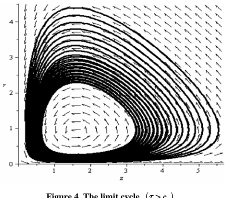
Example 2 Set

(

α σ ε χ ζ, , , ,

) (

= 1 3, 2, 3,1, 2

)

and τ =0.75. Then

0.7644280126

δ = .

this choice implies 0.1490319331 z

c = and ω =0.01248033802.

A limit cycle emerges in the

( )

r z, phase space (see,

[image:4.595.320.523.172.525.2]

Figure 4).

Figure 1. The bifurcation diagram.

Figure 2. The invariant torus.

Figure 3. The limit cycle

(

τ<cz

)

.

4

[image:5.595.60.285.82.280.2]

Figure 4. The limit cycle

(

τ>c_z

)

.

Interestingly, we can notice that [24] finds that local

indeterminacy occurs only when the condition τ <cz is verified, as in Example 1. However, the requirements for global indeterminacy are less stringent, since a pitch-fork-Hopf bifurcation can emerge even when the above condition does not hold. In contrast to [24], we may say that, global indeterminacy is likely to occur even if the pollution tax rate is either too low or too high, both of them possibly giving rise to free-riding problems, and an unsustainable use of natural resources, at the expenses of the long-run consumption pattern of future generations.

Therefore, if the initial condition on capital is chosen in such a way that system S gives rise to a toroidal motion, then a continuum of equilibria can depart from a given initial condition of the predetermined variable. Since this continuum of equilibria exists beyond the region relevant for the linear approximation of the dynamics in the neighborhood of the steady state, the result implies inde-terminacy of global nature [28].

Besides the result of global indeterminacy, the possibil-ity that the model can exhibit toroidal motion is of great interest also because the decomposition of the dynamics into phase/amplitude equations allows us to better under-stand the nature of the cyclical behavior of an economy where the intertemporal consumption is influenced by the use of natural resources, and the long run properties of the equilibrium become totally unpredictable.

4. Concluding Remarks

This paper shows that the growth model with endogenous discounting proposed in [27] presents global indetermi-nacy of the equilibrium in the full onset of the original ℝ3 structure. In detail, a study of the properties of the steady state in the vicinity of a codimension 2 pitchfork—Hopf interaction, allows us to demonstrate that global indeter-minacy can arise from plausible values of the parameters

in correspondence of the emergence of a trapping region with an invariant torus quasi-periodic dynamics. The me-thod innovates the literature in many aspects. First of all, it is the first time (to our knowledge) that a toroidal mo-tion is shown to emerge in simple two-sector endogenous growth models of the standard type. Second, the form of indeterminacy of the equilibrium we detect is obtained in the full ℝ3 dimension, which implies that, given any ini-tial value of the predetermined variable, there exists a continuum of initial values for the control (non-predetermined) variables in the ℝ2 submanifold.

REFERENCES

[1] J. Itaya, “Can Environmental Taxation Stimulate Growth? The Role of Indeterminacy in Endogenous Growth Mod- els with Environmental Externalities,” Journal of Eco- nomic Dynamics & Control, Vol. 32, No. 4, 2008, pp. 1156-1180. http://dx.doi.org/10.1016/j.jedc.2007.05.002 [2] I. Schumacher, “Endogenous Discounting and the Do-

main of the Felicity Function,” Economic Modelling, Vol. 28, No. 1-2, 2011, pp. 574-581.

http://dx.doi.org/10.1016/j.econmod.2010.06.014

[3] S. Smulders, “Environmental Policy and Sustainable Eco- nomic Growth: An Endogenous Growth Perspective,” De Economist, Vol. 143, No. 2, 1995, pp. 163-195.

http://dx.doi.org/10.1007/BF01384534

[4] A. L. Bovenberg and S. Smulders, “Environmental Qual- ity and Pollution-Augmenting Technological Change in a Two-Sector Endogenous Growth Model,” Journal of Pu- blic Economics, Vol. 57, No. 3, 1995, pp. 369-391. http://dx.doi.org/10.1016/0047-2727(95)80002-Q

[5] A. L. Bovenberg and S. Smulders, “Transitional Impacts of Environmental Policy in an Endogenous Growth Mod-el,” International Economic Review, Vol. 37, No. 4, 1996, pp. 861-893. http://dx.doi.org/10.2307/2527315

[6] P. Aghion and P. Howitt, “Endogenous Growth Theory,” MIT Press, Cambridge, 1998.

[7] A. Grimaud and F. Ricci, “The Growth-Environment Tra- de-Off: Horizontal vs Vertical Innovations,” Fondazione ENI Enrico Mattei Working Paper, No. 34, 1999.

[8] P. Schou, “Polluting Non Renewable Resources and Growth,” Environmental and Resource Economics, Vol. 16, No. 2, 2000, pp. 211-227.

http://dx.doi.org/10.1023/A:1008359225189

[9] K. Pittel, “Sustainability and Endogenous Growth,” Ed-ward Elgar, Cheltenham, 2003.

[10] M. V. Finco, “Poverty-Environment Trap: A Non Linear Probit Model Applied to Rural Areas in the North of Bra-zil,” American-Eurasian Journal of Agricultural & Envi-ronmental Sciences, Vol. 5, No. 4, 2009, pp. 533-539. [11] R. Perez and J. Ruiz, “Global and Local Indeterminacy

and Optimal Environmental Public Policies in an Econ- omy with Public Abatement Activities,” Economic Mod-elling, Vol. 24, No. 3, 2007, pp. 431-452.

http://dx.doi.org/10.1016/j.econmod.2006.10.004

Resources: The Different Roles of Capital and Resource Taxes,” Journal of Environmental Economics and Man- agement, Vol. 53, No. 1, 2007, pp. 80-98.

http://dx.doi.org/10.1016/j.jeem.2006.07.004

[13] S. Slobodyan, “Indeterminacy and Stability in a Modified Romer Model,” Journal of Macroeconomics, Vol. 29, No. 1, 2007, pp. 169-177.

http://dx.doi.org/10.1016/j.jmacro.2005.08.001

[14] C. Chamley, “Externalities and Dynamics in Models of Learning or Doing,” International Economic Review, Vol. 34, No. 3, 1993, pp. 583-609.

http://dx.doi.org/10.2307/2527183

[15] J. Benhabib and R. Farmer, “Indeterminacy and Increas- ing Returns,” Journal of Economic Theory, Vol. 63, No. 1, 1994, pp. 19-41. http://dx.doi.org/10.1006/jeth.1994.1031 [16] J. Benhabib J and R. Farmer, “Indeterminacy and Sector-

Specific Externalities,” Journal of Monetary Economics, Vol. 17, 1996, pp. 421-443.

[17] J. Benhabib and R. Farmer, “Uniqueness and Indetermi- nacy: On the Dynamics of Endogenous Growth,” Journal of Economic Theory, Vol. 63, No. 1, 1994, pp. 113-142. http://dx.doi.org/10.1006/jeth.1994.1035

[18] J. Benhabib, R. Perli and D. Xie, “Monopolistic Competi- tion, Indeterminacy and Growth,” Ricerche Economiche, Vol. 48, No. 4, 1994, pp. 279-298.

http://dx.doi.org/10.1016/0035-5054(94)90009-4

[19] J. Benhabib, Q. Meng and K. Nishimura, “Indeterminacy under Constant Returns to Scale in Multisector Econo-mies,” Econometrica, Vol. 68, No. 6, 2000, pp. 1541- 1548. http://dx.doi.org/10.1111/1468-0262.00173 [20] P. Mattana, K. Nishimura and T. Shigoka, “Homoclinic

Bifurcation and Global Indeterminacy of Equilibrium in a Two-Sector Endogenous Growth Model,” International Journal of Economic Theory, Vol. 5, No. 1, 2009, pp. 1- 23. http://dx.doi.org/10.1111/j.1742-7363.2008.00093.x [21] A. Ayong Le Kama and K. Schubert, “A Note on the

Consequences of an Endogenous Discounting Depending on the Environmental Quality,” Macroeconomic Dynam- ics, Vol. 11, No. 2, 2007, pp. 272-289.

[22] Q. Meng, “Impatience and Equilibrium Indeterminacy,”

Journal of Economic Dynamics & Control, Vol. 30, No. 2, 2006, pp. 2671-2692.

http://dx.doi.org/10.1016/j.jedc.2005.07.011

[23] T. Palivos, P. Wang and J. Zhang, “On the Existence of Balanced Growth Equilibrium,” International Economic Review, Vol. 38, No. 1, 1997, pp. 205-224.

http://dx.doi.org/10.2307/2527415

[24] A. Yanase, “Impatience, Pollution, and Indeterminacy,”

Journal of Economic Dynamics & Control, Vol. 35, No. 10, 2011, pp. 1789-1799.

http://dx.doi.org/10.1016/j.jedc.2011.06.010

[25] S. Wiggins, “Introduction to Applied Nonlinear Dynami- cal Systems and Chaos,” Springer-Verlag, New York, 1991.

[26] Y. A. Kuznetsov, “Elements of Applied Bifurcation The- ory,” Springer-Verlag, New York, 2000.

[27] J. Benhabib, K. Nishimura and T. Shigoka, “Bifurcation and Sunspots in the Continuous Time Equilibrium Model with Capacity Utilization,” International Journal of Eco- nomic Theory, Vol. 4, No. 2, 2008, pp. 337-355. http://dx.doi.org/10.1111/j.1742-7363.2008.00083.x

[28] E. Gamero, E. Freire, A. J. Rodriguez-Luis, E. Ponce and A. Algaba, “Hypernormal Form Calculation for Triple- Zero Degeneracies,” Bulletin of the Belgian Mathematical Society Simon Stevin, Vol. 6, 1999, pp. 357-368.

[29] E. Gamero and E. Ponce, “Normal Forms for Planar Sys-tems with Nilpotent Linear Part,” In: R. Seydel, F. W. Schneider, T. Küpper and H. Troger, Eds., Bifurcation and Chaos: Analysis, Algorithms, Applications, Interna-tionalSeries of Numerical Mathematics 97, Birkhäuser, Basel, 1991, pp. 123-127.

Appendix

Given the following system

( )

(

)

(

( )

)

( )

(

)

( )

(

)

(

( )

)

( )

(

)

( )

(

)

(

(

( )

)

( )

)

, , , , , , , , ), , , , , , , , , , , , , , k

k f k z k c z k k

c z k z k f k z k

u c z k z k c z k z k

τ τ λ θ δ

λ λ ρ τ λ θ τ δ τ

θ τ λ θ τ θρ τ λ θ τ

= − −   = _ + − _ = − +    (A.1) the associated Jacobian matrix is

(

)

( )

(

)

{

}

(

)

z k

c z k c c

z z z k

c z c c

P k c z c c

c u z c c

λ θ

λ θ

λ θ

ρ τ

λ ρ ρ τ λ ρ λ ρ

λ θ ρ λ λ ρ

∗ ∗ ∗ ∗ ∗ ∗ ∗ ∗ ∗  _{+ − − −}     _′  =_ − _ + − _{ }  _{− − + − − +}      J with

( )

(

)

( ) (

)

(

)

( )

( )

( )

Tr 2 B Det z k

z z k c

z k

c z

u z c

c z c P k

c P k

λ

λ

λ ρ τ

θ ρ λ τ ρ

ρ ρ τ λ

ρλ ∗ ∗ ∗ ∗ ∗ ∗ ∗ ∗ ∗ = + − = − + − ′ + _ + − _+ ′ = J J J

Consider a second-order Taylor expansion of the vector field in (A.1):

(

)

(

)

(

)

1 2 3 , , , , , , f k k _k f k f k λ θ

λ λ λ θ

θ

θ _{λ θ}

∗                _{= +}                       J       _  _{ }       _{   } (A.2) Where

(

)

(

2

)

2

₍

₎

(

₍

)

₎

2

1 2 2

1 , ,

2

c cc cc cc c kk zz k z kk z k z k

cc cc cc cc

u cc

f k f c z c z k c z k c z k

u u

θ

λ θ

ρ _{ρ θρ ρ ρ}

λ θ λ θ λθ θ

θρ θρ − +   = _ − + _ − − − − − −          

(

)

(

)

2

2 , , k kk 2

f k λ θ  = ρ − f kλ+ ρ λ_λ +ρ λθ_θ  

(

)

2

3 , , k 2

f k λ θ  =ρ θ ρ λθk+ _λ + ρ θ_θ

Assume now that system (A.1) undergoes a triple-zero eigenvalue structure, which allows us to make the fol-lowing change of coordinates

1 2 3 k w w w λ θ   _{ }     =   _{ }     _{ }   T    (A.3)

via an appropriate transformation matrix

1 1 1

2 2

3

0

1 0

u v z

u v z     =_{ }    

T (A.4)

whose columns represent the eigenvectors associated to the triple-zero eigenvalues (see [28]).

We are thus able to put (A.2) in a Jordan normal form

(

)

(

)

(

)

1 1 1 1 2 3

2 2 2 1 2 3

3 3 3 1 2 3

0 1 0 , ,

0 0 1 , ,

0 0 0 , ,

w w F w w w

w w F w w w

w w F w w w

          ₌  ₊          _{ }             (A.5) where:

(

)

(

)

(

)

2 3 1 1 3 2 2 1 3

1 2 3 2 3 1 1 1 3 2 2 1 3

2 1 1 2 1 2 2 1 3

1 , , i

v z f v z f v z f

F w w w u z f z u z f u z f

D

v f v f u v u v f

 _{− + +}    = _ + − − _  _{− + − +}    (A.6) with

2 1 1 2 3 2 1 3

D=v z −u v z +u v z 5.

Let us repeat the same procedure of above, and intro-duce a second transformation matrix:

2 0 1 0 0 0 0 δ ω ω −     = −_{ }    

B (A.7)

which allows us to put system (A.5) into the normal form suitable to describe the presence of one zero and a pair of pure imaginary eigenvalues:

1

1 1

2 2 2

3 3 3

0 0

0 0

0 0 0

f

x x

x x f

x x f

ω ω   −      _{ }  ₌  _{+ }      _{ }     _{    }   _{   }       (A.8) where

(

)

(

)

(

)

(

)

(

)

(

)

2 2 2 2 2 2

1 1 3 1 2 3 2 1 1 2 2 2 1 2 3 1 3 3 2 3

1

2 2 2 2 2 2

2 1 2 3 1 1 3 2 2 1 2 2 2 1 2 3 2 3 3 1 3

2 2 2 3 2 2

3

1 1 2 2 3 3 3 4 1 2 3

a x x c x x a x x x c x x x a x x c x x f

f a x x c x x a x x x c x x x a x x c x x

f _{b x x b x b x b x x x}

 _{− + + − + + −}        _{= + + + + + + +}           _{+ + + + +}        

which can be easily transformed in cylindrical coordi-nates:

3 2

1 2 3

2 2 3 2

1 2 3 4

2 2

1 2 3

r a rz a r a rz

z b r b z b z b r z

c z c r c z

θ ω

= + +

= + + +

= + + +

  

(A.9)

given x1=rcosθ, x2=rsinθ, x3=z (see [25]). Following [29], the truncated-amplitude system is de-rived from (A.9), keeping θ ω≈ :

2 2 3

ˆ ˆ

r=arz z=br − +z fz (A.10) where

1 2

ˆ a

a b

= − , ˆb= ±1,

and

(

4ˆ

)

3 2 _{z k}

a f

c z

ρ τ

= −

+ −

 

 .

A candidate for versal deformation of (A.10) is then

1

2 2 3

2 ˆ ˆ

r r arz

z br z fz

μ μ

= +

= + − +





with the following explicit values of

(

)

1 2

2 z k

c z

ρ τ

μ = + −

and

(

)

2 2

(

)

(

)

2

4 4

. 2

z k z z k c c k k z k kk kz k

c z u z c_λ c_λ f z z f f z

τ θ ρ λ τ ρ λ ρ δ τ ρ

μ

∗ ∗ ∗ _{ }

− − + − + − + _ − + + − − _