Using Box Jenkins Models to Forecast Mobile Cellular Subscription

http://dx.doi.org/10.4236/ojs.2016.62026

How to cite this paper: Siluyele, I. and Jere, S. (2016) Using Box-Jenkins Models to Forecast Mobile Cellular Subscription. Open Journal of Statistics, 6, 303-309. http://dx.doi.org/10.4236/ojs.2016.62026

Using Box-Jenkins Models to Forecast

Mobile Cellular Subscription

Ian Siluyele

1

_{, Stanley Jere}

2

1_{Zambia Information and Communications Technology Authority (ZICTA), Lusaka, Zambia} 2_{Department of Mathematics and Statistics, Mulungushi University, Kabwe, Zambia}

Received 29 November 2015; accepted 23 April 2016; published 26 April 2016

Copyright © 2016 by authors and Scientific Research Publishing Inc.

This work is licensed under the Creative Commons Attribution International License (CC BY). http://creativecommons.org/licenses/by/4.0/

Abstract

In this paper, the Box-Jenkins modelling procedure is used to determine an ARIMA model and go further to forecasting. The mobile cellular subscription data for the study were taken from the ad- ministrative data submitted to the Zambia Information and Communications Technology Authori-ty (ZICTA) as quarterly returns by all three mobile network operators Airtel Zambia, MTN Zambia and Zamtel. The time series of annual figures for mobile cellular subscription for all mobile net-work operators is from 2000 to 2014 and has a total of 15 observations. Results show that the ARIMA (1, 2, 1) is an adequate model which best fits the mobile cellular subscription time series and is therefore suitable for forecasting subscription. The model predicts a gradual rise in mobile cellular subscription in the next 5 years, culminating to about 9.0% cumulative increase in 2019.

Keywords

Mobile Cellular Subscription, Box-Jenkins Methodology, ARIMA Model, Autocorrelation Function, Partial Autocorrelation Function

1. Introduction

In Zambia, the penetration of information and communication technology (ICT) in general and mobile in par-ticularly, plays an important role in compilation of the national Gross Domestic Product (GDP). There are three (3) mobile cellular operators in Zambia with networks spanning land area of almost 602,090 Km2, representing 80% network coverage. In 2014, Zambia had 67.1% of subscribers from the mobile cellular subsector with revenue contribution of nearly K3.4 billion. At the end of December 2014 the population of Zambia was esti-mated at 15.1 million while mobile cellular subscription (MCS) was 10.1 million.

304

of the economy both at sectoral and aggregate levels. Therefore, the importance of investment in telecommuni-cation subsector is acknowledged world over. Globally, socio-economic effect and economic development due to improved telecommunication cannot be repudiated.

Time series modelling is an important part of every field. It provides both short and long term forecasting techniques. Effective implementation of forecasting techniques maximises the prospect of adopting optimum strategies. Literature shows that researchers have used both stochastic and deterministic models to model and forecast telecommunication data. However, stochastic models attributed to Box-Jenkins, the Auto Regressive Integrated Moving Average (ARIMA) models have been found to be more efficient and reliable even for short term forecasting than the deterministic models. Further, stochastic models are distribution-free as no assump-tions are required about the data or parameter hence the adoption of the forecasting methodology in this paper.

2. Method and Materials

The MCS data for the study has been taken from the administrative data submitted to the Zambia Information and Communications Technology Authority (ZICTA) as quarterly returns by all three mobile network operators (MNOs). The time series of annual figures for MCS for all MNOs is from 2000 to 2014 and has a total of 15 observations. Each observation (Xt) in the time series is sum total of subscriber for Airtel Zambia, MTN Zambia

and Zamtel i.e.

2000, , 2014

t t t t

X =α +β γ+ t= 

where,

t

α = number of subscribers for Airtel Zambia,

t

β = number of subscribers for MTN Zambia, and

t

γ = number of subscribers for Zamtel.

Statistical Analysis System (SAS) [1] and Microsoft Excel will be used to implement the stochastic models and graphical representations respectively.

3. Stochastic Modelling

The Box-Jenkins approach to forecasting was first described by statisticians George Box and Gwilym Jenkins and was developed as a direct result of their experience with forecast problems in the business, economic, and control engineering applications [2]. The Box-Jenkins methodology is a systematic process which is imple-mented by using an iterative process until an adequate model is achieved. The procedure is achieved by a step-by-step process of model IDENTIFICATION, SPECIFICATION, ESTIMATION, DIAGNOSTIC and FORECAST. The ARIMA has three parameters viz. autoregressive (p), differencing order (d) and the order of moving average (q). The generic Box-Jenkin models are denoted by ARIMA (p, d, q) given by

( )(

B Xt µ

)

θ

( )

B at

∅ − =

where, ∅, θ and a are autoregressive parameter, moving average parameter and residual respectively. The re-siduals are assumed to be iid1 Normal. Using the backshift operator/transformation the equation above, when d = 0, is expressed as

(

1

)

(

1

) (

1

)

1 1 1

1 p 1 p 1 q

p t p q t

B B X B B µ θB θ B a

− ∅ − − ∅ = − ∅ − − ∅ + − − − .

Also as

( )

( )

Constant t

t

B a X

B θ

= +

∅

where, at is a white noise process with mean 0 and variance σ2[3].

4. Measures of Forecast Accuracy

The statistics are used to compare how well models fit the time series. Akaike Information Criterion (AIC) and

1

305

Schwartz’s Bayesian Information Criterion (SBC) are some of the measures of accuracy of forecast that are widely used in SAS. Other measures used include Mean Squared Error (MSE), Mean Absolute Percentage Error (MAPE) and Mean Absolute Deviation (MAD). Forecast error is given by

(

)

( )

( )

Forecast Error FE_t =Observed Value O_t −Forecast Value F_t .

AIC and SBC are given by

( )

(

)

AIC= −2 ln L −k and SBC= −2 ln

( )

L +kln

( )

n .

Other measures of forecast accuracy are given by

(

)

2

1

MSE n Ot Ft

n

−

=

∑

,

1

MAPE 100

t n

t

FE O

n

=

∑

× and MAD FEt

n

=

∑

.

In these formulas, L is the value of the likelihood function evaluated at the parameter estimates, n is the number of observations, k is the number of estimated parameters and t=1, 2,,n.

5. Identification

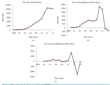
This is the foremost step of the Box-Jenkins process of time series modelling. A timeplot of the MCS is plotted in Figure 1(a) and checked for stationarity and invertibility using visual display of the ACF2 and PACF3 graphs.

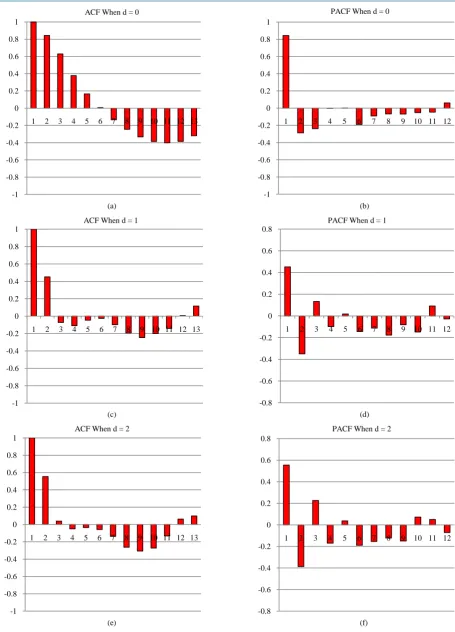
Figure 1(a) show that the MCS time series is not stable and therefore nonstationary. The nonstationary be-haviour is confirmed by the ACF and PACF plots in Figure 2(a) and Figure 2(b) below. Therefore some sort of transformation of the series is necessary to make it mean and variance stationary4. ARIMA models are designed to model stationary time series.

Converting a nonstationary time series to a stationary one through differencing (where needed) is an impor-tant part of the process of fitting an ARIMA model. Figure 1(b) and Figure 1(c) shows first order and second order differenced MCS series, respectively. The ACF and PACF plots are shown in Figure 2(c), Figure 2(d),

Figure 2(e) and Figure 2(f) below. ACF and PACF plots indicate that the first and second differenced MCS se-ries are stationary hence require further examination to establish the most suitable transformation for the MCS series.

Table 1 shows the details of various ARIMA models along the forecast accuracy measures. An ARIMA model with least measures of accuracy particularly the AIC and SBC is considered an efficient model for pre-diction. Therefore, for MCS time series, the ARIMA (1, 2, 1) is an adequate (best fit) model because it has the lowest values for AIC and SBC statistics.

6. Parameter Estimation

Table 2 shows the estimated parameters and the associated p-values at 5% level of significance. Only the auto-regressive parameter is significantly different from zero at 5% implying that the constant and the parameter for the moving average coefficients have little or no effect on the model.

The model variable and factors are given in Table 2. Hence, the mathematical form of the ARIMA (1, 2, 1) is

(

)

2

₍

₎

1 .

1 0.54647

t t

a

B X

B

− =

−

7. Diagnistic Check

Verification of goodness of fit of any model should include a test as to whether the residuals form a white noise process. Diagnistic check helps determine if an estimated model is statistically adequate. If the identified model passes the diagnostic tests, the model is ready to be used for forecasting. If it does not, the diagnostic tests

2_{Autocorrelation function.} 3_{Partial autocorrelation function.}

306

(a) (b)

(c)

[image:4.595.80.540.80.435.2]

Figure 1. Time plots for d = 0, d = 1 and d = 2 of MCS series.

Table 1. Measures of accuracy for selected ARIMA models.

ARIMA MODELS AIC SBC RMSE MAPE MAD

ARIMA (1, 1, 0) 422.68 423.96 725,927.03 79.94 500,531.81

ARIMA (1, 1, 1) 423.06 424.98 682,365.52 89.63 444,145.63

ARIMA (1, 1, 2) 425.07 427.63 679,685.36 87.49 436,179.08

ARIMA (2, 1, 1) 425.00 427.56 681,695.68 95.37 448,809.15

ARIMA (1, 2, 0) 404.26 405.39 1,086,694.05 93.33 772,506.46

ARIMA (1, 2, 1) 399.91 401.61 783,904.98 46.22 525,306.06

ARIMA (2, 2, 1) 400.35 402.61 770,165.27 87.90 530,058.84

ARIMA (2, 2, 2) 406.07 408.89 937,548.54 116.59 684,186.40

Table 2. Estimated parameter and significance tests.

TYPE Coefficient SE coefficient t-statistics p-value Lag

Constant 500,796 967,576 0.52 0.6048 0

MA (1) −0.99995 111.0529 −0.01 0.9928 1

AR (1) 0.54647 0.2761 1.98 0.0477 1

0 2000 4000 6000 8000 10000 12000

2000 02 04 06 08 10 12 14

M

C

S

'0

0

0

Time (Year) Time Plot of MCS Series

-1000 -500 0 500 1000 1500 2000 2500 3000

2000 02 04 06 08 10 12 14

M

C

S

'0

0

0

Time (Year) Plot of First Differenced MCS Series

-3000 -2000 -1000 0 1000 2000 3000

2000 02 04 06 08 10 12 14

Time (Year)

[image:4.595.87.538.467.631.2]

307

(a) (b)

(c) (d)

[image:5.595.83.539.77.710.2]

(e) (f)

Figure 2. The ACF and PACF plots for d = 0, d = 1 and d = 2 of MCS series.

-1 -0.8 -0.6 -0.4 -0.2 0 0.2 0.4 0.6 0.8 1

1 2 3 4 5 6 7 8 9 10 11 12 13 ACF When d = 0

-1 -0.8 -0.6 -0.4 -0.2 0 0.2 0.4 0.6 0.8 1

1 2 3 4 5 6 7 8 9 10 11 12

PACF When d = 0

-1 -0.8 -0.6 -0.4 -0.2 0 0.2 0.4 0.6 0.8 1

1 2 3 4 5 6 7 8 9 10 11 12 13 ACF When d = 1

-0.8 -0.6 -0.4 -0.2 0 0.2 0.4 0.6 0.8

1 2 3 4 5 6 7 8 9 10 11 12

PACF When d = 1

-1 -0.8 -0.6 -0.4 -0.2 0 0.2 0.4 0.6 0.8 1

1 2 3 4 5 6 7 8 9 10 11 12 13

ACF When d = 2

-0.8 -0.6 -0.4 -0.2 0 0.2 0.4 0.6 0.8

1 2 3 4 5 6 7 8 9 10 11 12

308

should indicate how the model ought to be modified, and a new cycle of identification, estimation and diagnosis is performed.

The Autocorrelation check for white noise of an ARIMA (1, 2, 1) model in Table 4 p-values at 5% level of significance as shown above indicates that the model is good because the residuals are a white noise.

8. Forecasting

Box-Jenkins approach to forecasting stationary time series is relatively simple. The forecast value of X_{t k}+ given all observations up until n the k-step ahead forecast is denoted by x kˆ_t

( )

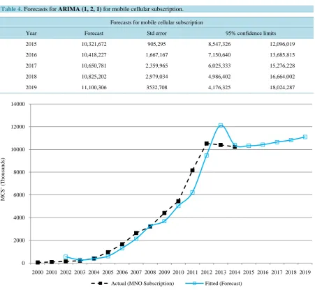
. Table 3 shows five year fore-casts for mobile cellular subscription using ARIMA (1, 2, 1). The trajectory of the forecasts from 2015 to 2019 is shown in Figure 3.

Table 3. Autocorrelation check for white noise.

To lag Chi-square DF Pr > ChiSq Autocorrelations

6 5.72 6 0.4558 0.555 0.040 −0.051 −0.035 −0.057 −0.139

[image:6.595.88.540.291.707.2]

12 18.63 12 0.0979 −0.263 −0.307 −0.272 −0.132 0.063 0.098

Table 4.Forecasts for ARIMA (1, 2, 1) for mobile cellular subscription.

Forecasts for mobile cellular subscription

Year Forecast Std error 95% confidence limits

2015 10,321,672 905,295 8,547,326 12,096,019

2016 10,418,227 1,667,167 7,150,640 13,685,815

2017 10,650,781 2,359,965 6,025,333 15,276,228

2018 10,825,202 2,979,034 4,986,402 16,664,002

2019 11,100,306 3532,708 4,176,325 18,024,287

Figure 3. Forecasting with ARIMA (1, 2, 1) for mobile cellular subscription.

0 2000 4000 6000 8000 10000 12000 14000

2000 2001 2002 2003 2004 2005 2006 2007 2008 2009 2010 2011 2012 2013 2014 2015 2016 2017 2018 2019

M

C

S

’

(T

h

o

u

sa

n

d

s)

309

9. Discussion

The ARIMA (1, 2, 1) is an adequate model which best fits the mobile cellular subscription time series and is

therefore suitable for forecasting subscription. The potential implication of this study is that by developing fore-casting models for predicting mobile cellular subscription in advance on a regular basis is to support internal de-cisions and planning as well as market communication. The subscription forecast baseline in this study uses his-torical data from Airtel Zambia, MTN Zambia and Zamtel. The study also provides a model to foresee and allo-cate appropriate resources to maintain a steady increase in mobile cellular subscription.

10. Conclusion

In this paper, the Box-Jenkins modelling procedure is used to determine an ARIMA model and go further to forecasting. The mobile cellular subscription data for the study were taken from the administrative data submit-ted to the Zambia Information and Communications Technology Authority (ZICTA) as quarterly returns by all three mobile network operators Airtel Zambia, MTN Zambia and Zamtel. The time series of annual figures for mobile cellular subscription for all mobile network operators is from 2000 to 2014 and has a total of 15 observa-tions. Results show that the ARIMA (1, 2, 1) is an adequate model which best fits the mobile cellular subscrip-tion time series and is therefore suitable for forecasting subscripsubscrip-tion. The model predicts a gradual rise in mobile cellular subscription in the next 5 years, culminating to about 9.0% cumulative increase in 2019.

Acknowledgements

The authors are thankful to Zambia Information and Communications Technology Authority (ZICTA) for pro-viding the data, Department of Mathematics and Statistics, Mulungushi University for using their resources and all the people who helped in making comments on this paper.

References

[1] SAS Institute Inc. (2014) SAS/ETS 13.2 User’s Guide: The ARIMA Procedure. SAS Institute Inc., Cary.

[2] Box, G.E. and Jenkins, G.M. (1994) Time Series Analysis: Forecasting and Control. 3rd Edition, Prentice Hall, Englewood Cliffs.