Basic Relationships in n Component Diabatic Flow EUR 3459

Hi ■TOPfflM

UR

345

:,5i#«

r \ i

Mw

i;

g

« F » * ι ' ' -f'

i

fcMH

_Kir

is;i

ir**·'·.'

CUI

M

•■"Χ',Ά

m

ATOMIC ENERGY COMMUNITY - EURATOM

' Jïr*j3»iit!v^ 'iii

m

It V W Idi »(»l»J ii»!'1 ¡ir

H'Wif! Nbi

*ί"ί·Μ

_•tilh

riff!

* a

_w

' M ' f J

H?*

lállt

î «y-TC

BASIC RELATIONSHIPS IN n-COMPONENT

il

_¿A"3

lit)

:.?;::.·1ΐ»ίΐ

_lì!

I»'»

M

im

DIABATIC FLOW

. WUNDT i t í

ktftisì ι · ·_{ï f } # } l} « . «J f* I

û

m

w«'

if1)'

pi«

II!

>»*<^iHr'f

iwftà

i ' j t t ' f » · * . » *

ftM

aPLHn

ifP

H ·1

i®£

mt

tmû

M l i i W l

• ; Î / I ·

ili

lililí

íhjHw'Ét.i

^uDrøM

fe«

' il«.!

M Í y.'

«A

m

iv,

i

'M i<vHr:i

ilS

f¡(il l<9

AãíS

Joint Nuclear Research Ce

affi

Research Reactors

m

»)';'%«

Hig Éifffl

imi

acting on their behalf :

Make any warranty or representation,

either the EURATOM Commission, its contractors nor any person

any warranty or representation, express or implied, with respect to the accuracy, completeness, or usefulness of the information con-tained in this document, or that the use of any information, apparatus, method, or process disclosed in this document may not infringe privately owned rights; or

Liity with respect to the use of, or for damages resulting Assume any liability with respect

from the use of any information, appar; disclosed in this document.

EUR 3459.e

BASIC RELATIONSHIPS IN n-COMPONENT DIABATIC FLOW by H. WUNDT

European Atomic Energy Community - EURATOM

Joint Nuclear Research Center - Ispra Establishment (Italy) Reactor Physics Department - Research Reactors

Brussels, April 1967 - 80 Pages - 1 Figure - FB 125

Relationships between the extensive quantities mass, volume, total energy, and momentum, and their related specific quantities, their densities, as well as their density currents, are compiled. On the basis of the "complete-mixing model" (the constituents may have different velocities, but fill each one the whole volume) and the conception of partial quantities, equivalent relationships are derived also for η-component flowing mixtures. With the aid of these expressions the general balances for mass, partial masses, momentum and energy (subdivided into internal, displacement, kinetic and potential energies) are established in three-dimensional, time-dependent coordinate-free partial

EUR 3459.e

BASIC RELATIONSHIPS IN n-COMPONENT DIABATIC FLOW b> H. WUNDT

European Atomic Energy Community - EURATOM

Joint Nuclear Research Center - Ispra Establishment (Italy) Reactor Physics Department - Research Reactors

Brussels, April 19G7 - 80 Pages - 1 Figure - FB 125

the consideration of chaotically numerous and transient internal boundary conditions at bubbles and droplets during boiling. Its drawback is t h a t slip effects, inter-phase viscosity, pressure drop, heat conduction, and the magnitude of the heat transfer coefficient for various flow-patterns cannot properly be seized. I t is proposed to combine some simplified equations with the necessary empirical correlation knowledges. The momentum equation proves to be unable for inclusion in a computer programme because of insufficient determination of the stress tensor for two phase flow. Details of the energy equation suffer equally from this difficulty so that, up to now, only its roughest statements could be applied.

A handy set of two equations is given and repeated in the conclusions which may be useful for calculating transients in heat exchangers and around boiling water reactor fuel elements, stability problems being excluded.

differential equation notation. Specialization to one-dimensional two phase flow is made.

The "complete-mixing model" is the only field theory t h a t permits to avoid the consideration of chaotically numerous and transient internal boundary conditions at bubbles and droplets during boiling. Its drawback is t h a t slip effects, intcr-phasc viscosity, pressure drop, heat conduction, and the magnitude of the heat transfer coefficient for various flow-patterns cannot properly be seized. It is proposed to combine some simplified equations with the necessary empirical correlation knowledges. The momentum equation proves to be unable for inclusion in a computer programme because of insufficient determination of the stress tensor for two phase flow. Details of the energy equation suffer equally from this difficulty so that, up to now, only its roughest statements could be applied.

E U R 3 4 5 9 . e

EUROPEAN ATOMIC ENERGY COMMUNITY - EURATOM

BASIC RELATIONSHIPS IN n-COMPONENT

DIABATIC FLOW

by

H. WUNDT

1967

Joint Nuclear Research Center Ispra Establishment - Italy Reactor Physics Department

their density currents, are compiled. On the basis of the "complete-mixing model" (the constituents may have different velocities, but fill each one the whole volume) and the conception of partial quantities, equivalent relationships are derived also for η-component flowing mixtures. With the aid of these expressions the general balances for mass, partial masses, momentum and energy (subdivided into internal, displacement, kinetic and potential energies) are established in three-dimensional, time-dependent coordinate-free partial differential equation notation. Specialization to one-dimensional two phase flow is made.

The "complete-mixing model" is the only field theory t h a t permits to avoid the consideration of chaotically numerous and transient internal boundary conditions at bubbles and droplets during boiling. Its drawback is that slip effects, inter-phase viscosity, pressure drop, heat conduction, and the magnitude of the heat transfer coefficient for various flow-patterns cannot properly be seized. It is proposed to combine some simplified equations with the necessary empirical correlation knowledges. The momentum equation proves to be unable for inclusion in a computer programme because of insufficient determination of the stress tensor for two phase flow. Details of the energy equation suffer equally from this difficulty so that, up to now, only its roughest statements could be applied.

CONTENTS

Preface page

1 . General form of "balances

2. Introduction of thermo­hydrοdynamic variables, homogeneous case

3. Relationships between thermo­hydrodynamic

variables, heterogeneous case

3.1. Integral quantities

3.2. Specific quantities

3.3. Densities

3.4. Current densities

3.5. Flow 'rates

4. Relationships of one­dimensional two­phase

flow

¿.(..1. Integral quantities

4.2. Specific quantities

4.3. Densities

4.4. Current densities

4.5. Relationships between fractions

4.6. Flov/ rates

5. The balance equations

5.1. Mass balance

5.2. Volume balance

5.3. Momentum balance

5.4. Energy balance

5.4.1. Homogeneous flow

5.4.2. Heterogeneous flow

5.4.3. Specialization to one­dimensional

two­phase flow

6. Conclusions

List of symbols

their density currents, are compiled. On the basis of the "complete-mixing model" (the constituents may have different velocities, b u t fill each one the whole volume) and the conception of partial quantities, equivalent relationships are derived also for η-component flowing mixtures. With the aid of these expressions the general balances for mass, partial masses, momentum and energy (subdivided into internal, displacement, kinetic and potential energies) are established in three-dimensional, time-dependent coordinate-free partial differential equation notation. Specialization to one-dimensional two phase flow is made.

The "complete-mixing model" is the only field theory t h a t permits to avoid the consideration of chaotically numerous and transient internal boundary conditions at bubbles and droplets during boiling. Its drawback is that slip effects, inter-phasc viscosity, pressure drop, heat conduction, and the magnitude of the heat transfer coefficient for various flow-patterns cannot properly be seized. It is proposed to combine some simplified equations with the necessary empirical correlation knowledges. The momentum equation proves to be unable for inclusion in a computer programme because of insufficient determination of the stress tensor for two phase flow. Details of the energy equation suffer equally from this difficulty so that, up to now, only its roughest statements could be applied.

CONTENTS

Preface page

1. General form of balances

2. Introduction of thermo-hydrodynamic variables, homogeneous case

3. Relationships between thermo-hydrodynamic variables, heterogeneous case

3.1. Integral quantities 3.2. Specific quantities 3.3. Densities

3.4. Current densities 3.5. Flow 'rates

4. Relationships of one-dimensional two-phase flow

4.1. Integral quantities 4.2. Specific quantities 4.3. Densities

4 . 4 . Current d e n s i t i e s

4 . 5 . Relationships between f r a c t i o n s

4 . 6 . Flov/ r a t e s

5. The balance equations 5.1. Mass balance 5.2. Volume balance 5.3. Momentum balance 5.4. Energy balance

5.4.1. Homogeneous flow 5.4.2. Heterogeneous flow

5.^.3. Specialization to one-dimensional two-phase flow

Two phase flow has, in particular in connexion with boiling heat transfer, become a field of very intense en-gineering research during the recent past. The interest has been stimulated by its appearance in boiling water re-actors and rocket engines as well as in several types of heat exchangers.

Correlation attempts to interprete numerous experimen-tal results and to predict the behaviour of designed plants are dispersed over well some thousands of papers. A very deserving textbook synopsis has recently appeared [1].

•My impression is that, despite of an almost "bewilder-ing abundance of data, the common theoretical foundations are to a certain deal fragmentary or even misleading.

In order to fill this gap this paper shall provide re-search workers with a systematic classification of basic relationships from hydrodynamics and thermodynamics that may be suitable for two phase flow investigations.

As it is irrelevant for our purposes to distinguish between chemically different "components" and chemically

identical but physically different "phases" of the same substance in a moving fluid, we speak, for convenience, of components only.

Moreover, most of the used definitions and relations are applicable to more than two components so that the no-tation is simplified by using the summation symbol over all components and giving the latter ones a current index i. In the case of pure phases, the number of participants is normally restricted to 2 due to GIBBS' phase rule so that

5

-The rigorous relationships derived in this paper are partly in a striking contrast to what is sometimes taken as a hasis in the literature to describe some two phase flow phenomena. It is for this reason that papers which further establish on such relations are intentionally not quoted. References are but made to such papers which deal with the derivation of the fundamental equations and which were thus of utility to prepare this paper itself.

In this sense, the scope of the present paper is li-mited. It cannot provide any new correlations nor can it finally clarify two phase flow mechanisms. The equations which will be derived show characteristic differences bet-ween homogeneous and heterogeneous flow, but are in fact

scarcely treated further; it is rather discussed why they cannot "be solved reasonably without certain specific ex-perimental informations.

This is to restrain engineers from too a vigorous em-pirical advance in some ases. The purpose of this paper

1. General form of balances *)

There are two methods of treatment of two phase flow and boiling heat transfer problems which do not exclude but should complement one another. The one is an empiri­ cal approach to explain isolated phenomena such as pres­ sure drop through pipes e.g., by means of dimensional analysis. The other method is the analytical one. This means that first the physical equations governing the

system are established. Then, in principle, if also the initial and boundary conditions are given, the solution should supply the complete subsequent system behaviour in space and time. Of course, such a sanguine expectation is, as always, quite academic as sooner or later a point will be reached where the rigorous continuation must be stopped

for a serious lack of informations about details.

"Nevertheless, just this "rigorous" approach shows in a coherent manner where and possibly how the gaps diould be filled by empirical informations of the first kind. True uncorstanding in sciences has almost ever been achieved in

this way.

Thus, we try to establish a set of partial differential equations describing the behaviour of a η-component flow with heat addition. This is, at least for two phase flow, not new, but our treatment will be somewhat more general than usual derivations, leading to better understanding.

*) _{' The "general" method of balances is followed also e.g.}

in [2] and [3].

The equations in question are, as known, the balances or conservation equations of mass , energy, and momentum, The thermodynamics of irreversible processes deals also with an entropy balance - the second fundamental lav/ is

the central problem of non-equilibrium thermodynamics -, but, as can be seen so far, no practical applicability

exists yet for boiling heat transfer problems.

We consider a volume V to which pertain the three ex­ tensive quantities M (mass), E (total energy), and Ρ (mo­ mentum). The amounts of those quantities can simply be added when joining two or more volumes to give the total quantity.

Let Y be any extensive quantity, then the following quantities will also be needed:

- the related "specific" quantity (per mass unit) y = Y/M - the related "Y-density" (per volume unit) py (with ρ =

mass density),

- the related "Y-current density" Φγ,

- the Y-flow rate through the closed surface of the given volume Qy,

- the Y-production density inside the volume oy.

By definition, Y is given by

Y = /pydV . (1.1) V

*)

' We prefer the physical notation of mass, not the engi­

by the production rate within, thus

dt dt v v

Qy is obtained by scalarly multiplying the Y­current den­

sity çEy (positive outwards) with the oriented surface dA

and integrating:

0γ = ­JÆy.dA ,

(1.3)

A

or, by GAUSS' theorem:

0γ = ­/­div ^ dV . (1.4)

V

Substituting (1.4) into (1.2) and cancelling the vo­

lume integration yields

£­ (py) = ­ div 3y + Ογ. (1.5)

3t

This is the differential "local" formulation of the

balance of any specific quantity y. It shall in the

following be specified to each one of our interesting thermo­hydrodynamic quantities. If y is a scalar, then

ΦΥ is a vector; if y is a vector, then φψ is a tensor

of second order

*)

' We denote, for typing convenience, scalars with arrow­

less characters, vectors with one arrow, and tensors with

Note that y, py, Φ*γ, and Cy are "locally" defined va­

riables or "field variables", whereas the other ones are

"integral variables", no more depending on position co­

ordinates.

We consider now the balance with respect to any velo­

city field φ, and move the integration volume dV with it.

The new current density with respect to this velocity field

is Φγ­pycp.

If we choose φ = ν, the "center of mass velocity" which

will be defined exactly in chapter 3, the mass pdV* re­

mains constant along the path. Instead of (1.2) we get

d _{= ­ M d L ­ nvv)­dÃ** + /c}

f^/pydV* = ­ / ( V pyv*)­cLÃ> + /cydV* , (1.6)

V* A* V­

where the asterisk suggests the moved volume. As pdV*

remains unchanged in time, the time derivation acts on y

only.

When applying once more GAUSS' theorem and cancelling

the volume integration, one gets

P 5 t ,= ­ d i v (% " pyv) + oy. (1.7)

One calls this the "substantial" formulation of the

*)

y­balance ' because the substance (mass) of the integra­

tion volume is held constant. The total differential ope­

rator d/dt changes to the "substantial differential ope­

rator" D/Dt which refers just to the mass velocity v,

*)

' The denotation "flow" formulation is too vague and

a.': no other one. ­his subtle remark becomes important

] ·. ter on. D/Dt is, as usual,

2_

=

|_

+ v

\

g r

„d ,

(1.8)

a. relationship .which can also be derived by eliminating

Cy f rem _ ( '■ . 3 ) ana (1.7). Due to the correction term v«grad, the independent position coordinate? remain the

11 ­

2. Introduction of thermo­hydrodynsmie variables:

homogeneous case

After having the general recipe to establish balances,

the only task is to specify correctly what is Φγ and o\r

in each case.

As already mentioned, we will substitute mass, total

energy, and momentum, resp., for Y. We will treat all

these quantities simultaneously and take the volume V it­

self as fourth extensive variable.

We first give a list of' the involved qua nti ties. The

nomenclature considers as much as nossible the recomman­

dations of the International Union for Pure and Apnlied

Physics (IUPAP), document U.I.Ρ 11 (S.U.U. 65­3) from

1965. Unfortunately, not seldom quantities coïncide which

usually have equal characters (e.g. ν for specific volume

and for velocity) so that side­step notations must be used.

The adopted units system is the "UiS­cystem where caloric ­"

units have already been transformed (e.g. Joules instead of

kilocalories). Conversion factors tire so avoided.

For each of the four blocks (see next page), the pro­

cedure is the same. In order to go from the "basic integral

Quantity to the corresponding specific quantity, one has

to divide by the mass M. The ratios are to be understood

as differential quotients. The specific Quantities are thus

suitable as field variables, and so do also the various

densities and. current densities. The "specific mass" χ for

a homogeneous body is, of course, simply unity, but for

more than one component the definition becomes non­trivial

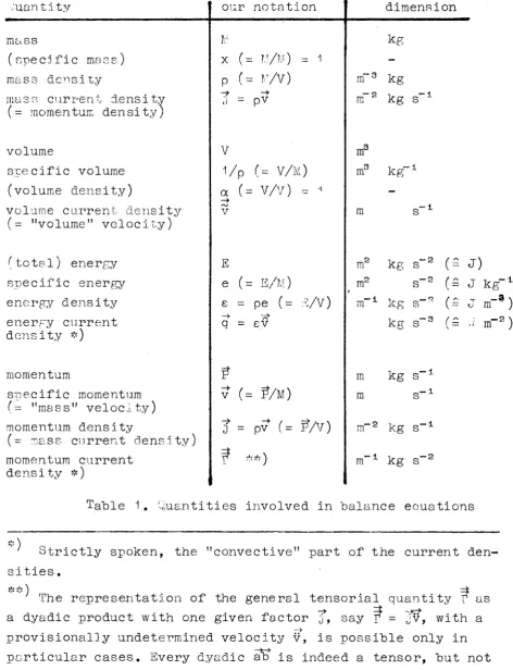
Quantity

mass

(specific mass)

mass density

mass current density (= momentum density)

volume

specific volume

(volume density)

volume current density (= "volume" velocity)

(total) energy

specific energy

energy density

energy current density *)

momentum

specific momentum (= "mass" velocity)

momentum density

(= mass current density)

momentum current density *)

Ol Γ χ

Ρ

V

ir ( = ( =

Vp

α —» v E e ε ­> q

f

­> v ->

f

( = ( = = ( = = . notation

=

M

A O

=

MA)

pv

(= v/?

= v/v)

= E/M)

pe ( =

-¿

εν

=

f/U)

pv ( =

s« )

= ^

ï)

— ­1

-Vv)

?/v)

m 3

m2 m3 m3 m ms m2 * m m m m"2 m dimension kg ­ kg kg kg" ­ kg kg kg kg kg kg s'1 1 s"1 s"2 s"2

S "

s"3 s­1 s­1 s­1 s­2 ( = ( =

(= J k g -1) ­3;

■ )

S)

m

Table 1. Quantities involved in balance eQuations

* )

' Strictly spoken, the "convective" part of the current den­

sities.

* * ) =*

The representation of the general tensorial quantity Γ as a dyadic product with one given factor j, say Γ = ¿ν, with a

­>

provisionally undetermined velocity v, is possible only in particular cases. Every dyadic ab is indeed a tensor, but not every tensor is a dyadic.

[image:18.595.79.552.76.693.2]

13

The respective third lines, the densities, are derived

from the integral quantities by division by the volume V.

Once more, the ratios should be consid.ered as differential

quotients. The direct way to obtain the densities is to

multiply the specific quantities with the mass density p.

Again, the "volume density" α assumes a non­trivial mean­

ing only for more*­component flow (see § 5,i>).

The various (convective) current densities are obtained

from the respective densities by multiplying the latter

ones with appropriate velocities. The right velocity is the

"mass velocity" ν in the case of mass, the "volume veloci­

ty" ν for volumes, the "energy velocity" ν for energies,

whereas an averaged "momentum velocity" does not exist for

more­component flow, unless in the one­dimensional (scalar)

case, as shall be shown in chapters 3 and 4. These notions

are unusual and shall thoroughly be explained in § 3.4.

All velocities are different for more­component flow. The

current densities are vectors for mass, volume, and energy,

but a tensorial quantity for momentum, which itself is al­

ready a vector.

The integral quantities "flow rates" (depending on time

only) are obtained according to' (1.3) and (1­.4) as

■•dA* = - / d i ·

Si

=

­ /pv­dA = ­ / d i v (pv)dV

r

k g

s ­ i ]

A

V

% = _{v . d X = / d i v ν dV}- > _{rm3 s "11}

>

• dÃ* = ­ /,

A V

•a?

= - I·

ν

ƒ dA·? = - { D i v Γ dV rm kg s "2]

Q = - /pev.dA = - / d i v (pev)dV fm2 kg s"3 1 ( = Γ.:νΊ)

A V

In the case of momentum, the differential operator

"Div" under the volume integral means the tensor diver­

gence, leading to a vectorial quantity, defined by

9Γ k ι

Div

•f .

Sx t

V ^ sr

k 2

V ^ sr

k3

9X;

· )

(2.2)

Concerning GAUSS' theorem for tensorial Quantities, one

finds in the literature (e.g. [5], p. 134)

/dA·? = /(Div­rÒdV,

(2.3)

A V

where the tensor Γ is the postfactor under the surface

integral, ^hen changing the factor sequence in this

This holds for rectilinear coordinates only. In the

case of curvilinear coordinates additional terms with

CHRISTOFFEL symbols occur (cf. e.g. r41, pr^. I65 and 177).

Our divergence has of course nothing to do v/ith the

sum at the main diagonal elements, which unfortunately is

also sometimes called the tensor divergence. The latter

quantity, a scalar invariant, should preferably be called

­ 15

non­commutative " s c a l a r " oroduet, the o r i g i n a i t e n s o r Γ must be r e p l a c e d by the transposed tensor* Γ' so t h a t an a l t e r n a t i v e n o t a t i o n to ( 2 . 3 ) i s

¡f-äJt = / ( D i v . ? ' ) d V = /(?.Div)dV. ( 2 . 4 )

A V V

In general, the above defined momentum flow rate ÖU is not parallel to the surface vector dA. The dimension

of Γ is, superficially considered, that of an energy, but

has nothing to do with that (different tensor order!).

The various "production densities" oy, which are lo­

cal auantities, represent in general the unhomogeneous

terms in the balances (see eq. (1.5) as well as eq.(l.7))

and do not follow from the already discussed quantities.

We denote them as follows:

mass production density σ,, ^m­3 kg s­ 1]

(volume production density) o,, [s­1 ]

energy production density ov, !"m­1 kg s~3]( = [W m"~3l)

'ill

momentum production density Offrn 2 kg s 21 .

Relationships b e t w e e n thermo­hydrodynamic variables;

heterogeneous case

3.1 .Jrrtegral jquan_t,±ti_e_s_

The truly interesting case is that our considered v o ­

lume consists of n components with current index i, which,

however, in our m o d e l , fill each the whole volume (so a s ,

e.g., air as a mixture of nitrogen and o x y g e n ) .

Let us then defi.ne "partial" quantities according to

partial masses

partial volumes

partial energies

partial momenta

ML :

VL :

El ■

ï*

= xLM

= aLV

= r LE

= x

L

« P

> (3.1.1)

where the non­dimensional Quantities xL, a1, γ , and γ1 may be called "mass fractions","volume fractions",

"energy fractions", and "momentum fractions", resp. Of

course:

η

xL

L=i

= 1;

\ ,

a1

ί=ι = 1;

η

YL

L=i = 1;

η '. zi

Χ

I =1

= Γ (unit tensor). '

(3.1.2)

'*) f \

' In the two component case (n = 2) with liquid and vapor,

ν

17

-Strictly spoken, the denotation of the (generally

assym-metric) tensors %L as "fractions" is not good, but shall

be kept for the moment. At the end of § 3.4, we will

discuss the general suitability of such tensorial quantities

We will further make the agreement that "partial" quan­ tities shall be denoted by upper indices, i.e. those quan­ tities whose sum gives directly - without any statistical

weight - the total quantity '. Thus

n n n n

Vi!

1

= M; V V

1

= V; V Ε

1

= Ε; Γ f

1

= F* . (3.1.3)

L = 1 I = 1 L = i ί = i

3.2.Specific quantities

When proceeding'to specific quantities, we must dis­ tinguish between

- "true" specific quantities, where the starting integral quantities are divided by their own (partial) masses Μ*, to be denoted by lower indices,

- "partial" specific quantities, where the starting in­ tegral quantities are divided by the t otal mass M.

' Provided that a conservation law holds for this kind

T h i s g i v e s

s p e c i f i c m a s s e s

" t r u e " " p a r t i a l "

ML/M' 1

1 · 1 * ) s p e c i f i c v o l u m e s .(—)L= VL/ML = —

Ρ PI

specific energies e-L = EL/ML

specific momenta · v; = PL/ML

χι- = Ml/M

(-)l= VL/M

Ρ

eL = E't/M

v' = ΡΫΜ

(3.2.1 AS in chapter 2, all Quotients should be understood as differential quotients; the above quantities are thus "field" quantities.

For the partial specific quantities holds

xl

L = 1 L = 1

η

P' e" = e vl

L = 1 I = 1

(3.2.2)

They can a l s o be e x p r e s s e d by means o f t h e f r a c t i o n s :

1 NI ■1

χι· 1 ; ( p ) = a1«­; eL = rLe ; v1 XL*v , ( 3 . 2 . 3 )

similarly to (3.1.1). It can easily be verified that the

occurring "fractions" for the specific quantities are

just the same ones as for the integral quantities.

•i. \ Ί Ι

' The relation (-5)9' L ; = Tjr is obtained by comparison with

­ 19 ­

Whereas the partial quantities are formal but suitable

quantities for computation purposes, the "true" quantities

have a physical meaning and numerical values independent

of the particular experimental situation. Apart from the

trivial quantity XL = 1, (0)1 means the specific volume

of each component or phase as it can be found in tables;

it is a state variable. For a given pressure e.g., it as­

sumes a well­defined constant value at saturation. This is

important, as then, for isobaric processes, (75)^ should

not be differentiated in the balance equation whereas

(p)1 should be differentiated.

e­L, the specific total energy which includes also the

kinetic energy and other part energies, cannot be read'from

tables, as it is the case for u(internal energy) or for h

(enthalpy), which are state variables. The relationships

between these energy forms are considered in § 5.4.

The true specific momentum v­L is easily understood to

be the true mass velocity of the component i.

In order to compute the partial specific quantities

from the true ones, one has always to multiply with the

mass fractions x'L = ML/Mf thus

xL

el = xLe t ?

xt = x^xL(= x M ; ( ¿ )L = xL( ¿ )L = jL­ ;

vL = xLvL . (3.2.4)

By substituting these relations into (3.2.2), one has

(the first expression being trivial):

Π ΓΙ Π II

) χ1 = 1; ) . χ1(τ\)ϊ = h / . x l ei = ei / . X'L^L = ^ ·

(3.2.5)

/ ■ ~ ' L · vPyi

Here'we have found the recipe how to compute the quan­

1 ­>

tities —, e, and v, resp., which we must consider to be

representative for the mixture, from the corresponding

"true" values of the components.

The second relation of (3.2.5) must, later on, be com­

pared, with the­ averaging rule for the density p,to be de­

rived in (3.3.6).

The third equation, applied tc two phases, is the ener­

gy averaginr rule fcr flowing wet steam. An equivalent

rule holds for the entropy s. However, the well­known rules

for the internal energy u and for the enthalny h (cf. Γ3],

p. 163) are restricted to mi\vterres with no relative motion

of' their components. This may be understood by considering

that each component carries a kinetic energy k¡_ which, in

irreversible processes, may be partly or completely de­ stroyed leading to supplementary internal energy of the

joined body. Thus, for quantities without conservation law,

such as for u, h, or k, 2 u'L = Σ x^u^ / u, etc. Obviously,

before establishing averaged Quantities, all components must be

thought to have already joined one another.

The last eauation (3.2.5) finally gives the instruction

how to compute the center of mass velocity ν we had al­

ready spoken about in chapters 1 and 2.

By comparing formulas (3.2.3) and (3.2.4), the follow­

ing relations between the "fractions" a'1, γ'1, and γ} with x'L are obtained:

a1·­ = xL. ( ­ )L; Yle = xLeL; yL.v = xLvL .

­ 21

lhe last relation indicates that the linear transfor­

mât ­>

mation described by χυ turns the vector ν into the di­

rection of vL .

The steam fraction x of wet steam is also (correctly)

called "quality" in thermodynamics, α is the "void frac­

tion", γ has no proper name. It is cautioned not to call

χ a quality, not even for one­dimensional flow where

it reduces to a scalar, though its value is particularly

easy to measure at the end of a test path. "Quality"

suggests a material property that χ is not because of the

involved velocity situation.

Further relationships between fractions, specialized

to two phase flow, will be given in chapter 4.

3.3. Dens ities

Let us now proceed to the various densities. Once more,

we have to distinguish between "true" and "partial" den­

sities, according to whether we divide the integral quan­

tities by the individual partial volumes V'L or by the

total volume V.

mass densities

volume densities

energy densities

momentum densities

. Pt

a t

ε ι

-*·

3l

" t r u e "

= M*L/Vl

= VL/ Vl = 1

= Et/Vi­

= FVVL

" p a r t i a l "

pt = ML/V

at = VL/V

ε1 = EL/ V

ÎL =

P-/V

­he sum of the partial densities is the total density

in each case:

n n n

"3>i ­3>

(3.3.2) '( pL = p; / , CL1 = 1; ¿ , ε1 = ε; ' , D ­ J

Γ=ι L=i t=i ί=ι

Like (3.1.3·), we find

pL = xLp; aL = αι·1; ε1 = τ1ε: îTL = v.L ·î . (3.3.3)

Once more, the seme fractions as for th,e integral and

the specific Quantities occur. This is obvious as the

partial densities can also be computed from the partial

specific Quantities by multiplying the latter ones by p:

pL = pxL; a1 = p(£)1: ε1 = pel ; j>L = pvL . (3.3.4)

The partial densities are commuted from the known true

densities by multiplying the latter ones with the volume

fractions a'L = V'L/V:

pL = aLp­L; a.L = aLa¡,( = α1); ευ = α1 ει; tl = aLj\ .

(3.3.5)

T h i s can be summed t o y i e l d :

η η η η

> i \ ï Λ \ ï \ i -* ->

; , α PL = ρ; / , ocL = 1 ; /_ , aLe t = ε ; / ay 2χ. = d .

L =ι Γ=ΐ i. =ι L=i

23

-By comparing (3.3.5) with (3,5.5), one can relate xL, γ1 , and γ} to aL :

χςρ = aLpL ; - ; γιε = «le-L ; χ1· ?8 α17ί. (3.3.7)

The representation of the component densities by the specific quantities and the mass densities of the respec­ tive components is given by:

J ει = pteL ; J, = pLvt (3.3.8)

; al = oHhl ; et = p ^ ; f- = p<<v\ . ^ ' 5 ' ^

Comparison of the second relation of (3.2.5) with the f i r s t relation of (3.3.6) gives

ρ = ¿ , alp t = — . (3.3.10)

t = i

V ? !

l—i Pt

L = i

In the case of η = 2, this yields a coupling between

ocL and xl by means "of the known pj,. This shall be con­

sidered in more generality in the following chapter. For

η > 2, similar equations are not obtainable. Notice that

3.4.Current densities

As in chapter 2, we multiply the various densities with appropriate velocities in order to get the nertaining

current densities. From the demand that once more the par­ tial quantities should sum up to the total quantity, those velocities can be computed.

In order to calculate first the "true" component current densities, we multiply the respective true densities with

the only available true velocities vL , namely

?t = Pivi ; vL = αιη = vL ; qL = ef.vL ; Γι = jftn .

(3.4.1)

Here, in the case of a homogeneous component, we may

in-deed represent r-L as a dyadic product .

The "true volumetric velocities" vL of components are

equal to the respective mass velocities v-L..

To convert true densities to partial densities, the

former ones are to be multiplied by aL. As a consequence,

the current densities behave equally:

DL = pLvt ; vL = aLvi ; qL = eLvL ; V1 = iLvL = pLvLvL.

(3.4.2)

The chosen factor sequence is arbitrary as j\v-L = pi.v\v\

25

-For the mass current density which is identical with

the momentum density j, this was airead?/ stated in ( 3...·.-.).

But for the first time it comes out that the partial

—>

"volumetric" velocities v1 of the components are not

eaual to the respective ΑΛ = x^vj,.

By summing up the partial quantities we get

η η η η

/ . ] = . ! ; / vL = ν : / q1 - q ; / Τ1 = Γ .

ί=ι Γ=ι 1=1 1=1

("Λ.3)

If we substitute the expressions (3.3.3') into (3.4.2) and add according to (3.4.3), w.e find

η η η

>/ ( xLv¡, = pv ; 1 · / auvL =

p / x"vL = pv ; i · / orvL = ν ; ε / Y"V­L = εν ;

ί = ι t = 1 I =1

η

/ . (Χ. · 3 ) ν ι = Γ / any ¿ν ­, (3.4­.4)

L = l

where the right hand sides are taken from table

*)

; As no associative law holds for this kind of multinli­

=$·

cation, it is impossible to turn the linear operator γ1

-ï ­» ­>

The "mixture" velocities in question are thus found to be:

V

mass : ν = / _ xLv-L

Γ=ι

η

* V

t-volume: v = ,· α V[

ί =ι >

7?

V :

=

T.

r

l

ïi

1 = 1

energy:

momentum: "ν" not separately er is ting in general.

Cï.h.5)

The statistical weights to construct them are just the original ratios known from the integral quantities.

The following relations may also be useful (to deduce

from 3.4.5 with 3.2.3):

π π η

V

L ~»

­*

V ,1,U

1 á

Vt"»·

/ xLvL = v ; / (p) vL = ρ v ; > eLvL =

ί=ι l=i L=i

η

but / vLvL / vv . (3.4.6)

­ 27

It remains still to give relationships between partial

and total current densities, for which we write ad hoc

­, ι. _ vL · j ; ν = β ·ν · Q = δ ·Ρ · Γ = ι!/ · Γ .

(3.4.7)

The f i r s t r e l a t i o n i s a l r e a d y known from ( 3 . 3 . 3 ) , l a s t e o u a t i o n ; χ1 c o u l d t h u s d i r e c t l y be i n t r o d u c e d .

Eor t h e o t h e r r e l a t i o n s , we s u b s t i t u t e (5.^.5) i n t o

(3.4.2), 1 e a d i n g t o

>: p v i = XL ,p v ; aLV{, = ßL' V ; YLev-L = ôL« e v ;

(χι·Ϊ)νι = ψ1· Γ , (3.¿+.8)

w i t h

η η η ­ η

^

=*t

?

V &

3

V

Ä

?

V

/ XL = I : / ßL = I : / ôL = I ­

/ . x

L

=

Γ

; ζ , ß

L

= ï

; Ζ . δ

1

= Ι ;

¡_ . ψ

= ï

.

t = i L=i ί=ι ί=ι

( 3 . 4 . 9 )

The s i g n i f i c a n c e of ßL, oL, and . ψ1 i s p u r e l y a c a d e m i c , a s f a r a s t h e y cannot be computed unambiguously from t h e

-> ~

v a r i o u s g i v e n v e c t o r s v , v , e t c .

* ) =£}

This brinrs us to the problem of the utility of such

tensorial quantities in connection with η­component flow,

as already mentioned in § 3.1. We do not speak here about

the tensors in the general balances treated in chapter 2,

such as the momentum current density Γ, or the dyadic

products occurring for rL. They all have a real physical

meaning.

The question is rather what is about the "fractions"

=*L ^L 3l %

X » ß » δ , and ψ . Let us discuss e.g. the­last equation

of (3.2.3), which may be considered as definition for γ}.

The vectors vu and. ν are all known. Assume for the mo­

ment m­dimensional vectors, then we have just m eouations

for a certain i, whereas the "unknown" tensor γ1 contains

m2 elements. Thus, equations of this kind are solvable

only for m = 1, i.e. for scalers. For m >_ 2, no unambiguous

solution exists. None of the tensors in question has there­

fore a reasonable meaning except for one­dimensional flow

where they reduce to scalars. In more­dimensional formu­

lations, they must completely be avoided..

3.5 o£'low_ra tes

Although integral quantities have nothing to do with

the differential formulation of balances, we bring them

here for completeness. This is in particular in order

- 29

Similarly to eqs. (2.1), we get partial flow rates

% = _ (

/rjt.dÃ* = -

_{- ( (}

jW'D'tâ

A

0, _V - ; v

/ v

Ll

.di? = ·- /(ft.^.dsr

«dA

A'

JE

= - íq^.dÃ* = - /(c^-q)-dA

A

-H.

/cLA«rL = - /< / ά Α · ( ψι· Γ ) ,

>

J

( 3 . 5 . 0

where the relations (3.4.7) have been used.

=* =* 4: 3·

In view of the unprofitableness of χ , β, δ1, and ψ1

4. Relationships for one­dimensional two phase flow

'When considering two phase flow, in particular water

and steam, through a straight pipe, it is rather obvious

to simplify the balance equations by restriction to a

single axial coordinate. All vectors and tensors reduce

to scalar quantities, omitting the components pertaining

to the other coordinates. The objections arising from

such a neglect shall be treated only in chapter 5.

Here we will compute the formulas of the nreceding

chapters for n = 2 phases. The fractions of vapor shall

be denoted, as usual, by χ, a, etc., without index, those

of liquid by (1­x), (1­oc), etc. For the indices used, ν

means vapor, 1 means liquid. For upper indices we write *

instead of v, and ' instead of 1.

The elementary volume V is a disk with area A and any

(insignificant) thickness dz. ¿11 integral quantities

can equally be considered as quantities per unit length.

"e give formulas for the practical use without much

comment, referring simply to the relations of preceding

chapters where they have been taken from, in square brackets,

[3.1.1]:

M' = xM

V » = αν

E' = γΕ

Ρ' = XP

M' = (l­x)M

V' = (l­a)V

E' = (ΐ-γ)Ε

Ρ' = (ΐ-χ)Ρ Ν

> (4.1.1)

31

4.2.Specific Quantities

"true" specific quantities [3.2.1 ]

(1)

=

ï!

=

i_

^p;v M' p„

E|

V ~ M'

ν ρ*

ν ~ M*

rl)

- Ii _ 1

vp;l " M' Pi

v.

M'

EL

M'

> (4.2.1)

"partial" specific quantities [3.2.1], [3.2.3], [3.2.4]:

X

Φ

e"

=

=

=

M' M

V M

E ' M

_ vi _ α _ / I N

. β _

M

= Ye = xe

= χν = xv.

( 1 - x ) = MJ _M

Φ'

e'

ν '

V ' ' M

Ξ ' " M

Ρ ' ' M

M P K Χ ΑΡ;1

= ( ΐ - γ ) β = ( l - x ) e1

>

( 1 - Χ ) ν = ( ΐ - χ ) νχ

specific quantities of mixture Γ3.2.5]

χ 1-x

— +

ν Pi

= xe + (l-x)e, _ν

v 1

ν = xvy + (1-X)V1

> (4.2.3)

relations between fractions [3.2.61

α χ Y χ X χ V V V V 1-α 1-x 1_y 1-x 1"X 1-x Ρ Pi

!i

e V > (4.2.4) 4.3.Densities

"true" densities Γ3.3.1] , [3.3.8]

pv =

ε =

V

Κ

=

M" V '

E '

V ' =

Ρ '

V*

-- ρ e

κν ν

ρ ν *ν ν

Μ_ V'

Ε'

ν, κι η \ (4.3.1)

εΊ , - ρ e.

EL

"partial" densities [3.3.1], [3.3.31, [3.3.4], Γ3.3.5Ι

» ..

M_l

V

E'

= X p = OCR

V

e * = 7j—_V = γε = αε = pe* = ρ "e

v v

V " = X3 = α ϋν = p v · = p ' vv

ρ'

=ψ-

=

(1-x)

=

0-α)

_Pi

EJ

V = ( 1 - γ ) = ( ΐ - σ ) ε1 = pe' = p'e^ \ " ( 4 . 3 . 2 )

y = — = ( l - x ) j = ( l - a ) j1 = pv' =

p'v-mixture densities [3.3.6]:

GO

co

Ρ = ο.ρν + ( ΐ - α ) ρ1

pe = ε = «ε + (ΐ-α)ε1 = o:pvev + (l-a)p1e1

ρν = j = a jv + ( l - a ) jx = «pvvy + (l-a)p1v1

> (k.3.3)

relations between fractions Γ3.3.7Ι

N

χ

α

Y a.

y

a

v Pve V pe

Ρ v Hv v

pv

1-x P l

A-a " p

1-Y εχ

1-α " ε

1- X 3\

1-α j P lel

pe

P lvl

pv

> ( 4 . 3 . 4 )

4.4.Current densities (now scalars)

true" current densities [3.4.1]

J = ρ ν

uv * v ν

ν = ν

ν ν

h

= Pi

v

i

vi = vi

> 0 = ε ν = ρ e ν q_ = ε , v., = ρ, e., v.,

'V v v Hv v v ^ 1 1 1 μ1 1 1

Γ = J v = ρ Ve

V V V V V Γ1 = Vi = Ρΐν1

J

(U.4.1)

"partial" current densities [3.4.2 ], [3.4.7] :

j ' = p ' vv = x j = a jv j ' . = p ^ = ( l - x ) j = ( l - a ) ^

v " = α νγ = βν = a vv v ' = ( ΐ - α ) νχ = ( ΐ - β ) ν = (l-oOvL

q ' = ε * νγ = ôq = a q ^ q ' = ε ' ν1 = ( l - ô ) q = ( l - a ) q -L

>

Y" = j ' v v = ψΓ = α Γν Γ ' = j , v1 = ( ΐ - ψ ) Γ = ( ΐ - α ) Γ2

J

mixture c u r r e n t d e n s i t i e s Γ3.4.4"':

j = a jv + ( l - a ) j1 = a pvvy + ( l - a ) p1v1 = ρΓχνγ + ( ΐ - χ ) νχ] = pv

ν = a vv + ( 1 - a ) ^

q = aqv + ( l - a ) a1 = a p ^ e ^ + ( l - a ) p1e1v1 = pe [ γ νγ + ( ΐ - γ ) ν1] = pev

Γ = αΓ„ + (1-α) ΓΊ = αρ„ν2 + Η - α ) ρ ν | = ρνΓχνγ + ( ΐ - χ ) ν . , ] = ρνν '

>

ν ν

( 4 . 4 . 3 )

definition of velocities Γ3.4.ΡΙ:

ν = xvv + ( ΐ - χ ) νχ

ν = a vy + ( ΐ - α ) νχ

ν = γ νγ + ( ΐ - γ ) ν1

>

ν = Χ% + (1- χ ) νχ

* )

J

n

Here, and only i n t h i s one-dimensional' c a s e , v g e t s a meaning: v = / xlvc

1=1

00

en

4.5.Relationships between fractions

In contrast to formulas (4.2.4) and (4.3.4), the re­

lations can also be given without recourse to mixture

properties, but with the "true" phase properties only.

For this purpose, we define the following ratios bet­

ween "true" specific Quantities

­ the specific volume ratio ξ

­ the specific energy ratio η

(Vp)y _ PjL

(Vp)

1

p

v

V

V V

­ the specific momentum ratio S =

(= velocity ratio or slip ratio) 1

> Í4.5.1)

For a given saturation pressure, ξ is numerically

known. The same is but not true for the slip ratio S, as

it is not built by state variables, nor for η, as e is

no state variable.

Let

ρ Ρ *)

= u + k = h ­ (τ0„ + k ; en = u­, + k, = h­, ­ (ñ). + k,

r ν ν ν vP'v v' 1 1 1 1 vP'l 1

(4.5.2)

where k and k. are the· specific kinetic

ν 2 1 · 2

energies and u , u, the specific internal energies of the

components. Then

u +k ­ (un+k, ) u ­u..

ν ν 1 1 Λ ~ ν 1 Λ

η = : ­ ι .

Ul+ kl U­

(4.5.3)

Λ, \ "t-J

­ 37 ­

u ­υ... is the evaporation heat at constant volume (con­

v 1 v

s tant ρ). In most cases, k­L is negligible against u­L ;

nevertheless, (4.5.3) is rigorous only for the components

at rest.

Similarly,

η

hv­(p/p)v+kv­[h1­(p/p)1+k1]

^ ­ ( ρ / ρ )χ+ ^

h ­h,

­ 1 s ­ 2 — ¿ ­ 1, (k.5.k)

where h ­h­, is the evaporation heat at constant pressure p,

and the so­called expansion energy p/p is omitted.

It is further to be noticed that both h, and u, are

known except for an additive constant. For saturated wa­

ter of 0 C, h, is, by convention, equated to zero. The

enthalpy difference h, (and u, , too) is free from such

arbitrariness and thus by far more suitable than η for

theoretical purposes.

From (4.2.3), (4.2.4), (4.3.3), and (4.3.4), the fol­ lowing relationships are easily obtainable

χ =

α =

Y =

α

α + ξ(ΐ-α)

Υ

ΐ£.

ξχ + (1-χ)

ηχ ηχ + (1-χ)

Sx

Χ :: Sx + (1-χ)

Λ ξ γ ηα - Γ + +

η ( ΐ ·

η(ι·

ηα

ξ ( ι ·

Sa

- γ )

-Υ)

-α)

Χ

Χ + S(1-x)

1χ_

ξχ + S(1-X)

m

ηχ + s(i-x) sy

Sa + ξ(ΐ-α) Sy + η(ΐ-γ)

OC I

;

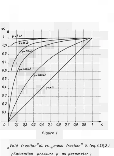
0,9

Ofl

0,7

0,6

0,5

0,4

0,3

0,2

0,1

ι ■

Ρ»

1

­Iah ~ρΜ(

/?·

ΙΨ*Μ

1

"¡Γ^

5oJ>

)0«L(*

1

ρ « i o

1 »at

/pc.

rik

—^ — ^ - i ' » ■

O I 0,1 0,2 0,3 0,4 0,5 0,6 0,7 0,6 0,9 7 X

Figure 1

» ))

..Void fraction oC vs. mass, fraction X (eq. 4.5.5,2 )

[image:44.595.152.542.109.642.2]

­ 39 ­

4.6.Flow rates

"partial" flow rates [3.5.1]

M

- ( ■

XJ cLA

Qv =

°^ =

Qp =

­ /ßv dA A

­ /Ôq dA A

­ /ψΓ dA A

= ­ /(l­x)j dA A

Q¿ = ­ /(l­ß)v dA

A

«έ

. . f

/(l­ô)q dA

Op = ­ /(l­*)r dA . A

> (U.6.T)

The integrations must be extended over flow cross sec­

tions A perpendicular to the flow direction. But as a

variability of the integrands normal to the flow axis can­

not be considered in a consistent one­dimensional theory

(unique position coordinate is z ) , the above expressions

degenerate to

« 4

-« , ­

«i =

< *

-­ XdA

­ ßvA

-

mA

­ ψΓΑ

^ =

^v =

%

< *

-­ (1.

­(1.

­ (1

­ (1

­X)JA

­β)νΑ

­ô)qA

­ψ) ΓΑ

If the left hand expressions are divided by the total

flow rates Q„, 5L·, Q„, Qp, resp., (see 2.1., specialized

to one dimension), the area A and the current densities

j, v, q, and Γ, cancel in all cases so that follows

Q"

II

X ­ o

¿M

*

"V

v

o*

_E 0

%

\

mass flow rate ratio

β = — volumetric flow rate ratio

energy flow rate ratio

ψ = — momentum flow rate ratio.

>

J

(4.6.3)

All these quantities are integral quantities, thus

foreign to a differentially formulated theory. They are

results of the processes inside a test distance and have

a meaning only at its end.

In particular, the relatively easily measurable quan­

tity χ, frequently called "quality" in the literature, is

not suitable to be used in our theory. Obviously, any cor­

relation between integrai! and locally defined (field­)

quantities is without meaning, e.g. between χ and a, or

similar ones, as it can be stated between two local quan­

­ 41

5. The balance equations

5.I.Mass balance

After the lengthy preparations of chapters 2, 3, and 4,

we will now use the general balances, either in "local"

form (1.5) or in substantial form (1.7), and specify the

general current densities iL and the production densi­

ties Oy.

In the case of mass, y is the "specific mass", i.e.

unity (see table 1 ) . The current density ãL is ~$ = pv,

anõ., without mass sources, aM = 0.

This gives

■— = ­ div pv. (5.1.1)

The substantial formulation (1.7) is not'directly

suitable in the mass case. But by applying (1.8) on the

density ρ and considering (5.1.1) one finds

=£ = ­ ρ div ν ,

(5.1.2)

Dt

another well­known formulation of the continuity equation.

We now proceed to the balance of partial masses, y is

here xL (partial mass per total mass, cf. 3.2.1), and

<£h = jL = pLv\ (cf. 3.4.2). This can all be chosen quite

■ Thus, according to (1.5):

a(pxL) ?PL L­> ? / c , ,x

8 t ~ = 9t~ = ­ G 1 V Ρ vt + °M » (5.1.3)

or substantially (1.7):

DxL

Dt = ­ d i v (plV{, ­ p'Lv) + oj, , ( 5 . 1 Λ )

n

τ —·

\

v/here ) σλ = 0 .

ί : M t =1

The expression pL(v{,-v) will also appear later on. It

is the excess of the partial current density over the correction due to the movement of observation point and may be called "(mass-) diffusion current density"

«Í1 = pl(vL­v) (5.1.5)

of the component i.

η

Of course, ) J*1 = 0.

l=i

Eq. (5.1.3) may herewith also be written as

43

-When specializing the formulas to one-dimensional two phase flow, we have

at

+ V 9z + Ρ

Έ =°

3v (5.1.7)

dp' dp' 9νη , - .

9t" + Vl θ ζ ~+ Ρ 9z~ = Va» * )

9t ν 9z 9z

9p' 9p' 9v^ „

+ ν — + ρ' τ-* = oM(z,t) .

?

(5.1.8)

The equations are not independent one from the others, as the sum of eqs. (5.1.8) gives just ec. (5.1.7).

In the one-dimensional treatment, the overall suita­ bility of which for boilinr; rhenomena investigations is

not assured, the partial densities pL can be replaced by

the known true densities pt. At the same time the vapor velocity ν may be reduced to 'the liquid velocity v., by

introducing the slip ratio S(z,t). The suitability of this measure in view of a solution of the system is also doubtful.

Eqs. (5.1.8) transform to

9v-9t

O f V η

[Ρι(ΐ-α)] + νχ — ΓΡι(ΐ-α)] + Ρι(ΐ-α) — *

¿(z.t)

■ΓΤ ( ρ α) + S(z,t)vn -ζ- (ρ α) + ρ α ­r— rS(z,t)v,^

3t ν"ν ' ν ' ' 1 3ζ ν rv "ν 8ζ χ * ' \

ft

■

a

L

(z

'

(5.1

>

t)

or, if ρΊ and ρ are,constant for constant saturation

pressure,

3 a

3t Vl 3z"oa + (',-a)

9V. 3z

σ ^ ζ , ΐ )

, N 3a 3S , . Sv-, . o¿¡(z,t)

+ ^ + S t z . t ^ ­ + α Γ νχ ­ + S(z,t) g ^ ] = ­ ^ ι a

ν

>

(5.1.10)

The state variable α acts as a dimensionless mass

s u r r o g a t e , ­mnhasis is to b e laid on the fact that S(z,t) enters into the equation as a foreign b o d y . The r e p l a c e ­ m e n t of ν _ by 'h' reveals to be only a p s e u d o ­ s i m p l i f i ­

cation as long as t h e slin ratio S is n o t known as f u n e ­ st

tion of ζ and t '

The right­hand inhomogeneous terms must b e otherwise

p r o c u r e d (from the energy equation, as w e shall s e e ) .

5.2 .Volu.me_ balance

Though resulting only in trivialities, the formal p r o ­

cedure shall also b e applied to our v o l u m e quantities, in

order to show the overall consistency.

The specific volume is y = 1/p, and the volume current

density is <&, = v, according to table 1 .

*)

45 ­

Thus, the local formulation yields

§£ "1" = ­ div ν + σν = 0 (5.2.1)

which means that no geometrical volume storage is

possible. The substantial formulation reads

Ρ Dt 'õ' = " d l V (v ­ v) + Cy (5.2.2)

or

1 Dp _>

­ r κ? = + div ν, (5.2.3.)

Ρ Dt

when cancelling div ν due to (5.2.1). This is just eq. (5.1.2).

Notice the important difference between ν and the

special velocity v.

The partial volume balances may be omitted.

5.3. Momentum_balan.c e

As the energy balance requires some additional thermo­

dynamic considerations, we will first investigate the momentum balance.

This balance is called NAVIER­STOKES' equation of move­

ment in hydrodynamics. Thus, in the case of homogeneous

one­component flow, we should arrive at some well­known

notation, but the heterogeneous flow will lead to a more

sophisticated formulation, as we shall see.

' Besides, the source can be evaluated to be cy = ) Oy = ) Ojy/Pi

According to our general procedure, we choose for y the specific momentum v, a vector; see table 1.

The momentum current density, to be read from eq. (3.4.4), is

V

_(χ

₁

_.Τ)ν\

V

_{Ρ vivi}

1=1 1=1

This is the pure convection part ano. is not complete. As well known, particles of real fluids interact mutually by pressure and viscous forces resulting in a momentum transfer. This additional (and preponderant) momentum current density is described by the stress' tensor

P+P xx

P

zx

Ό

xy

P P+P yx yy

ρ _xz

yz

P P+P _{zy * - zz}

*)

[kg m"1 s"2] (5.3.1)

The normal pressure ρ ' is superimposed by "viscous

pressures" pjt which, according to STOKES, are given by

/3V/.X 9ν/,Λ

pj l -μ

K-ér

₃₁ 1 +

"ãj '

!

- l^'

ôdiv ν

Ji

dl

j = x,y,ζ

ι = χ,y,ζ .

(5.3.2)

s¡0

' For the description in non­Cartesian coordinates,

cf. [7].

"' This pressure p(t,r) is one of our system variables

­ 47

The tensor Π is symmetric: ρjι = Ptj. μ is the usual

dynamic viscosity and μ' is the so­called "second visco­ 2

sity parameter" which is sometimes specified to ­μ' = =■ μ,

The latter relation is however rigorously valid only for

monoatomic gases (ENSKOG 1917). We shall make no use of

the definition (5.3.2). It is further convenient to use

the viscous part of Π separately by subtracting the sca­

lar pressure ρ from the diagonal elements:

ff*= ff - p ?

Ρ _{^xx *xy} Ρ "O _"xz

Ρ Ρ Ρ

yx yy yz

P P P

■^zx ^ z y ­*ζζ

It may be anticipated that Div ·? = 0 so ti _that

(5.3.3) ­

Div

_{(P?) =}

grad p.

(5.3.4)

A momentum production σ=>· may be caused by external for­

ces proportional to mass, such as gravity. Let ft [m/s2]

be this force (per unit mass) on the i· component, then

σ ^

u

>

i

?

t [kg m"s s­ 2] (5.3.5)

In the case of gravity which we will consider exclu­

­> ­»

sively, ft is equal to g, the free­fall acceleration vec­

tor, so that

Substitution of these expressions into eq. (1.5) gives

the local formulation

or

ft (pv) =

­ Div(r+n) + pg ,

(5.3.7)

•|t (pv) = ­ Div Γ ­ grad ρ ­ Div Π* + pg. (5.3.8)

In order to reduce the current density to the given velocity field v, we must subtract pvv from ilU = Γ+Π

(see eq. ( 1 . 6 ) ) . Thus, the substantial formulation accord­ ing to eq. (1.7) is

T \ —> —»

Ρ Dt = ~ D i v ' r + Dj­v«(pvv) ­ D i v π + pg, (5.3.9) o r

p ^ = ­ Div(r­pvv) ­ grad ρ ­ Divïï* + pg Κ (5.3.10)

Unless for homogeneous (one­component) flow, ψ is not

equal to pvv, as can be seen from the last expression

in (3.4.4).

' The term D i v ( r ­ p w ) can also be written as D i v / v t J1

L = 1

with JL defined by (5.1.5). This illustrates the origin

49 ­

The vector Div·(pvv) is parallel to v, as every ex­

pression of this kind is parallel to the last vector in

the dyadic product:

­...■rh ­" .-■',,,: -'· ι,"' ',, fr'ïpqioofîl o í

D i v (pat?) = (grad ρ·?)"? + (ρ div a)"t? +p (a«Grad)"b* .

(5.3.11)

In contrast to this, ß i v r is in general not parallel to v, because it cannot be expressed in the form Div.(pvv)

as we have seen. Thus, the additional term Div·(Γ­pvv)

changes both magnitude and direction of the time deri­ vative vector ^v/Dt against the case of homogeneous flow.

The above formulations 5.3.7 to 5.3.10 may be consi­

dered as an extension of the usual NAVIER­STOKES' ecua­

tion to heterogeneous flow.

The elements of the tensor Π* are, as shown in

eq. (5.3.2), themselves functions of the velocity compo­

nents and a material property μ, the viscosity. This is

already true for the simpler case of laminar motion. For

a turbulent flow, the stress tensor is superimposed by

the tensor Π. ^ of turbulent "apparent" viscosity, the

element ajk of which is ρ vjvk. vj etc. are Cartesian

components of the turbulent oscillation velocity ν' , and

the bar means a time average '. Their computation as well

as their measurement are extremely difficult; the theore­

tical statements (PRANDTL's mixing length etc.) are by

far unable to predict correct results in complex cases

like ours.

* i

' The method applies to quasi­stationary turbulence. For

macroscopically rapidly changing velocity fields, the

What is still more serious is the fact that the ele­

ments of both tensors n* and Π, , refer of course to

11 turb.

a homogeneous fluid. The important open question is how

to incorporate two or more entirely different viscosi­

ties μ5_ into the stress tensor, and which velocities

should reasonably be applied.

Here the complete­mixing­model suggests some idea but

not yet a solution. It is obvious that only a unique pres­

sure field p(t,r) is physically possible, and not a set

of different but completely overlapping (true) pressure

fields p­L(t,r) . The same must be true for the tensor

n*(t,r) which is a unique one for the mixture. No dif­

ferent tensor components ρ . can occur because the con­

^xy,i

stituents are undistinguishible as concerns their po­

sition.

Hence the "mixture" friction tensor Π* must entirely

refer to mixture velocity components and a "mixture vis­

cosity" μ. If μ is a material property for homogeneous

fluids, the same can hardly be true for a mixture, as the

effect of fricción between ­ really ­ separated components i and k must be considered in any way. This latter cross­

—» —>

effect however depends on both velocity fields vL and νκ,

strictly spoken on V­L­VK.

This reasoning reveals that the relatively simple

STOKES' statement (5.3.2) is insufficient for more­com­

ponent flow and may not be used. The effective viscosity

for slip­flow must be higher than that computed from mo­

lecular­statistical theories for gas and liquid mixtures

at rest (see e.g.[8]).

' "Partial" pressures pL = aLp can of course be consi­^