http://dx.doi.org/10.4236/ojfd.2013.34039
Direct Numerical Simulation of a Jet Issuing from
Rectangular Nozzle by the Vortex in Cell Method
Tomomi Uchiyama1, Masahiro Kobayashi2, Shouichiro Iio3, Toshihiko Ikeda3 1EcoTopia Science Institute, Nagoya University, Nagoya, Japan
2Graduate School of Information Science, Nagoya University, Nagoya, Japan 3Faculty of Engineering, Shinshu University, Nagano, Japan
Email: [email protected]
Received October 3, 2013; revised November 3, 2013; accepted November 10,2013
Copyright © 2013 Tomomi Uchiyama et al. This is an open access article distributed under the Creative Commons Attribution Li- cense, which permits unrestricted use, distribution, and reproduction in any medium, provided the original work is properly cited.
ABSTRACT
Direct numerical simulation of a jet issuing from a nozzle having a rectangular cross-section is conducted. The vortex in cell (VIC) method, of which computational accuracy was heightened by the authors in a prior study, is used for the DNS. The aspect ratio of the nozzle cross-section is 15, and the Reynolds number based on the shorter side length of the nozzle exit is 6700. The turbulence statics, such as the mean velocity and the turbulence intensity, are favorably com- pared with the experimentally measured results. The behavior of the large-scale eddies as well as the development of the turbulent flow is also confirmed to agree with the measurement. These indicate that the authors’ VIC method is suc- cessfully employed for the DNS of rectangular jet.
Keywords: Rectangular Jet; Vortex in Cell Method; DNS; Vortical Structure
1. Introduction
Vortex in cell (VIC) method [1] is one of the simulation methods for incompressible flows. It discretizes the vor- ticity field into vortex elements and computes the time evolution of the field by tracing the convection of each vortex element using the Lagrangian approach. The La- grangian calculation markedly reduces numerical diffu- sion and also improves numerical stability. Thus, the VIC method is eminently suitable for direct numerical simulation (DNS) and large eddy simulation (LES) of turbulent flows, and various results have been reported. Cottet and Poncet [2] applied the VIC method for the wake simulation of a circular cylinder, and captured the streamwise vortices occurring behind the cylinder. Cocle
et al. [3] analyzed the behavior of two vortex systems
near a solid wall, and made clear the interaction between two counter-rotating vortices and the eddies induced in the vicinity of the wall. Chatelain et al. [4] simulated
trailing edge vortices, and visualized the unsteady phe- nomena caused by disturbances. These studies are con- cerned with time-developing free shear flows. But the VIC method has not been applied to turbulent flows bounded by solid walls, which are closely related with the turbulent friction and heat transfer.
The authors [5] performed the DNS of a turbulent channel flow, which is a representative example of wall turbulent flows. When applying the existing VIC method, the oscillation of the flow increased with the progress of the computation, and eventually the computation col- lapsed. This was caused by the fact that the consistency among the discretized equations is not ensured. This was also because the solenoidal condition for the vorticity is not fully satisfied. To overcome such problems of the existing VIC method, the authors [5] proposed the im- proved VIC method. The authors [5] also applied the improved VIC method to the DNS of the turbulent chan- nel flow. The DNS highlighted that the time evolution of the flow is fully computed and that the statistically steady turbulent flow is favorably obtained. It also demonstrated that the organized flow structures, such as streaks and streamwise vortices appearing in the near wall region, are successfully captured and that the turbulence statistics, such as the mean velocity and the Reynolds stress, agree well with the existing DNS results.
ticity field promises to be usefully applied to the simula- tion. But the VIC method has been scarcely used for the jet simulation.
The objective of this study is to search for the applica- bility of the authors’ VIC method [5] to the DNS of jet flows. The DNS of a jet issuing from a nozzle having a rectangular cross-section is performed by the VIC me- thod. The jet velocity field was experimentally inves- tigated by Iio et al. [6]. The aspect ratio of the nozzle
cross-section is 15, and the Reynolds number based on the shorter side length of the nozzle exit is 6700. The DNS results, such as the mean velocity and the turbu- lence intensity, are favorably compared with the meas- ured ones. The behavior of the large-scale eddies as well as the development of the turbulent flow is also con- firmed to agree with the measurement. These indicate that the authors’ VIC method is successfully employed for the DNS of rectangular jet.
2. Vortex in Cell Method
2.1. Vorticity Equation and Orthogonal Decomposition of Velocity
For an incompressible flow, the vorticity equation is gi- ven by
2t
u u
(1)
where u is the velocity and
u
is the vorticity. According to the Helmholtz theorem, the velocity u is the sum of the curl of a vector potential ψ and the gradient of a scalar potential :
u (2) when ψ is postulated to be solenoidal or 0, the curl of Equation (2) yields the vector Poisson equation for ψ:
2
(3) Substituting Equation (2) into the continuity equation and rewriting the resultant equation, the Laplace equation for is obtained:
2 0
(4) Once ψ and have been computed from Equa- tions (3) and (4) respectively, the velocity u is calcu- lated from Equation (2). The vorticity in Equation (3) is estimated from Equation (1). The vortex in cell (VIC) method discretizes the vorticity field into vortex elements, and calculates the distribution of by tracing the con- vection of each vortex element.
It is postulated that the position vector and vorticity for the vortex element p are xp
xp,yp,zp
and p,respectively. The Lagrangian form of the vorticity equa-
tion, Equation (1), is written as [7]:
d d p p t xu x (5)
2
d d
p
p p p
t u x x x
(6)
When the position and vorticity of a vortex element are known at time t, the values at t t are computed from the Lagrangian calculations of Equations (5) and (6). In the VIC method, the flow field is divided into computational grid cells to define ψ, and on the grids. If is defined at a position xg
xg,y zg, g
, the vorticity is assigned to xg, or a vortex elementwith vorticity is redistributed onto xg
v N
g p g p g p
p p
x x y y z z
W W W
x y z
(7)
where x, y and z are the grid widths, and Nv is the number of vortex elements. For the redistribution function W , various forms are presented [7]. To sup- press the numerical dissipation, a high-order scheme, which preserves the three first moments of the distribu- tion, twice continuously differentiable and symmetric, is employed for W :
3 2
2
1 2.5 1.5 1
( ) 0.5 2 1 1 2
0 2 W (8)
Equation (8) was used for the simulations of time-de- veloping free shear flows [2-4]. The DNS of a turbulent channel flow was also successfully performed with Equa- tion (8) by the authors [5].
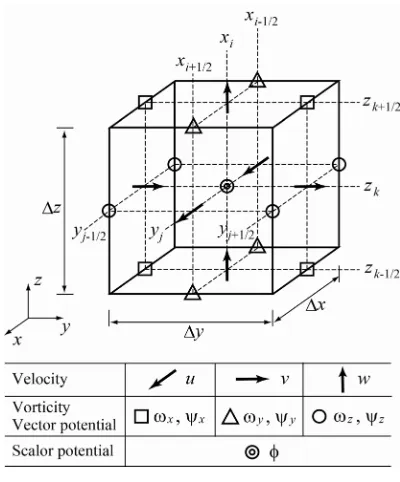
2.2. Discretization by Staggered Grid
For incompressible flow simulations, the MAC and SMAC methods solve the Poisson equation, which is derived from the equation for pressure gradient and the continuity equation. These methods employ a staggered grid to ensure consistency among the discretized equa- tions, and to prevent the numerical oscillation of the so- lution. The staggered grid would appear to be indispen- sable for discretizing the Poisson equation for ψ and the Laplace equation for , which are derived in the VIC method. However, staggered grids are not readily accommodated in the existing VIC method.
Figure 1. Staggered grid.
2.3. Correction of Vorticity Field
In the VIC method, the vorticity field is discretized into vortex elements, and the field is expressed by superim- posing the vorticity distributions around each vortex ele- ment. The superposition is performed by Equation (7). The resulting vorticity field r does not necessarily sa-
tisfy the solenoidal condition [7]. Denoting the vorticity satisfying this condition by s
u
, r is repre-sented as [3]
r F s
(9) where F is a scalar function. Equation (9) corresponds to
the Helmholtz decomposition of r.
Taking the divergence of Equation (9), the Poisson equation for F is obtained:
2
r F
(10) Calculating F from Equation (10) and substituting into
Equation (9) gives the recalculated vorticity s [3].
This correction for vorticity needs to solve the Poisson equation, which increases the computational time. To reduce this additional cost, the authors [5] have proposed a simplified correction method.
The uncorrected vorticity, r, is linked to r through
Equation (3). Taking the divergence of Equation (3) and substituting Equation (10) into the resultant equation, the following relations are obtained:
2 2 r r F (11)Unlike the assumption for the solenoidal condition of , the following equation for a non-solenoidal vorticity
is derived from Equation (11).
r F
(12)
Using r to calculate r from Equation (3), and
determining r from Equation (4), the curl of ur trans-
forms as follows:
2r r r
r r r s F u (13)
Equation (13) demonstrates that the curl of the veloc- ity ur calculated from r yields a vorticity s that
satisfies the solenoidal condition. If the vorticity is re- calculated by Equation (13), or the vorticity is corrected immediately after calculating the velocity by Equation (2), the discretization error in the vorticity is completely removed and the flow dynamics are accurately simulated without solving the Poisson equation, Equation (10). It should be noted that the staggered grid is required for rendering the transformation in Equation (13) applicable to the corresponding discretized equations.
2.4. Simulation Procedure
Given the flow at time t, the flow at t t is simu- lated by the following procedure:
1) Calculate the change in the strength of each vortex element defined on the grid, or calculate the vorticity
p
from Equation (6).
2) Calculate the convection of each vortex element, or calculate the position xp from Equation (5).
3) Redistribute the vortex element onto the grids, or calculate the vorticity on the grids by Equation (7).
4) Calculate the vector potential from Equation (3). 5) Calculate the scalar potential from Equation (4). 6) Calculate the velocity u from Equation (2). 7) Correct the vorticity, or calculate the corrected vor- ticity from the curl of u.
3. Simulation Conditions
The DNS of an incompressible jet issuing from a nozzle having a rectangular cross-section is performed. The jet velocity field was experimentally investigated by Iio et al.
[6]. The computational domain is shown in Figure 2. The shorter side length of the nozzle exit is w, and the
longer side length is 15w. The x-axis is along the jet
centerline, while the y- and z-axes are parallel to the shorter and longer sides of the nozzle exit respectively. The computational domain consists of a cubic region of
40w40w40w. It is resolved into uniform grid cells of
Figure 2. Rectangular nozzle and computational domain.
respectively. The jet velocity at the nozzle exit is U0, and the Reynolds number based on w and U0 is 6700. Table 1 summarizes the simulation conditions.
The boundary conditions are given as follows: Within the nozzle exit, a uniform and constant velocity U0 is imposed.
0
0
, , ,0,0
0, 0, 0
0
x y z
x y z
u u u U
x x U (14)
The non-slip condition is adopted on the wall at x0,
on which the nozzle exit is mounted. 0
0, 0, 0
0
0, ,
x y z
x y z z y
x x
u x u x
u (15)
The velocity gradient is set at zero on the other bound- aries. For example, the following conditions are imposed at y 20w.
2 2 0
0, 0
y z
x y z
y
x x
x y z
(16)
The time increment t is w
100U0
. A fully de- veloped flow was obtained at a time of 200w U0. The time-averaged velocity and the turbulence intensity were acquired in the period from 250w U0 to 550w U0.4. Results and Discussion
4.1. Instantaneous Flow Fields
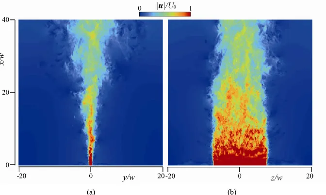
The instantaneous distribution for the absolute value of
Table 1. Simulation conditions.
Direction x y z
Nozzle size - w 15w
Domain length 40w 40w 40w
Grid cell number 400 400 400 Grid width w/10 w/10 w/10 Nozzle outlet velocity U0 0 0 Reynolds number wU0/v 6700
Time increment Δt w/(100U0)
the velocity u for the fully developed jet is shown in Figure 3. The distribution on the central cross-sections of the jet is presented. Figure 3(a) shows the result on the x-y cross-section at z = 0 parallel to the shorter side of
the nozzle exit. The potential core disappears at x/w ≒
2.6, as mentioned later. Thus, the jet spreads in the lateral direction downstream of the disappearing point, indicat- ing the momentum diffusion in the direction. The distri- bution on the x-z cross-section parallel to the longer side
is shown in Figure 3(b). It should be noted that the jet width becomes slightly narrower as the streamwise dis- tance increases.
The vorticity components z and y at the same
instant as Figure 3 distribute as plotted in Figure 4, where the distributions on the jet central cross-sections are presented. The shear layers originate from the shorter and longer sides of the nozzle exit, and the turbulent flow rapidly develops just after the collapse of the shear lay- ers.
Figure 5(a) shows the velocity on the jet central cross- section parallel to the shorter side of the nozzle exit, where the distribution near the nozzle is plotted. To make the distribution more understandable, the velocity 0.5U0 is subtracted. On the shear layers originating from the longer sides of the nozzle exit, large-scale eddies occur at
x/w ≧ 2.2. The eddies are non-axisymmetric around the
jet centerline. They change into eddies having various scales as the streamwise distance increases. Figure 5(b) presents the flow field visualized experimentally by illu- minating an alcohol mist with a laser light sheet [6]. The image clearly visualizes the occurrence of some large- scale eddies on the shear layers as well as the rapid change of the flow into turbulence. It is confirmed that the DNS successfully resolves the flow development including the occurrence and collapse of large-scale ed- dies.
4.2. Time-Averaged Velocity
(a) (b)
Figure 3. Instantaneous velocity distribution of fully-developed jet. (a) x-y cross-section at z = 0; (b) x-z cross-section at y = 0.
[image:5.595.128.467.318.515.2](a) (b)
Figure 4. Instantaneous vorticity distribution of fully-developed jet. (a) ωz on x-y cross-section at z = 0; (b) ωy on x-z
cross-section at y = 0.
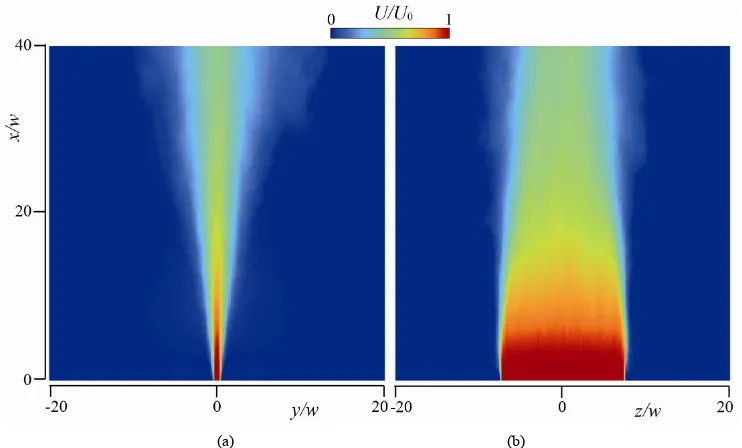
central cross-sections as shown in Figure6. On the x-y
cross-section parallel to the shorter side of the nozzle exit, the jet diffuses more in the lateral direction at x/w ≧ 3 as
the streamwise distance increases. On the x-z cross-sec-
tion parallel to the longer side, however, the jet width becomes narrower at x/w ≧ 3 in the downstream direc-
tion.
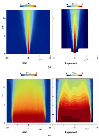
Figure 7 compares the time-averaged velocity com- ponent U obtained by the DNS with the measured re- sult of Iio et al. [6]. A constant temperature hot-wire
anemometer was employed for the measurement. It is found that the time-averaged flow features, such as the behavior of the potential core and the change in the jet width, are favorably grasped by the DNS.
The time-averaged velocity component U distributes
on the y-z cross-sections as shown in Figure8. The sec- tions are parallel to the nozzle exit. Figure 8(a) presents the DNS result. With increasing streamwise (x) distance,
the jet spreads more in the y-direction. But it contracts
gradually in the z-direction. These distributions agree
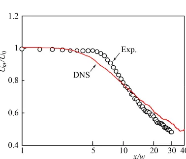
well with the measurements depicted in Figure 8(b). The time-averaged velocity on the jet centerline Um changes as a function of the distance from the nozzle as shown in Figure 9. The potential core exist until x/w =
(a) (b)
Figure 5. Flow field visualized on x-y cross-section at z = 0. (a) DNS; (b) Experiment.
(a) (b)
Figure 6. Distribution of time-averaged axial velocity. (a) x-y cross-section at z = 0; (b) x-z cross-section at y = 0. behavior of the large-scale eddies depends on the veloc-
ity and turbulence intensity distributions within the noz- zle exit. Some fluctuations exist in the velocity measured at the nozzle exit, and affect the velocity decay on the jet centerline through the occurrence and collapse of the
[image:6.595.112.483.423.647.2]DNS Experiment (a)
[image:7.595.140.455.78.510.2]DNS Experiment (b)
Figure 7. Comparison of time-averaged axial velocity near nozzle. (a) x-y cross-section at z = 0; (b) x-z cross-section at y = 0. The half widths along the shorter and longer sides of
the nozzle exit, by and bz respectively, change as
shown in Figure 10. by becomes larger as the stream-
wise distance increases. But bz reduces slightly. These
DNS results agree almost with the measured ones [6].
4.3. Turbulence Intensity
Figure 11 presents the jet axial component of the turbu- lence intensity urms . The distributions on the jet central
cross-sections are plotted. On the x-y cross-section par-
allel to the shorter side of the nozzle exit, urms is larger
at x/w ≦ 10 on the shear layers originating from the
longer sides of the nozzle exit. On the x-z cross-section
parallel to the longer side, urms takes the maximum
value on the shear layers from the shorter sides.
In Figure 12, the turbulence intensity urms obtained
by the DNS is compared with the measurement [6]. Though
rms
u of the DNS is larger near the nozzle as well as on
the shear layers originating from the shorter side of the nozzle exit, the trend of the distribution agrees well with the measurement.
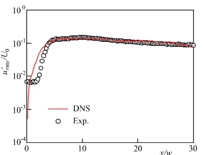
The turbulence intensity on the jet centerline varies as shown in Figure 13. The turbulence intensity of the DNS hardly coincides with the measurement [6] near the noz- zle (x/w ≦4.2). This may be caused by the fact that the DNS ignores velocity fluctuations at the nozzle exit and the boundary layer on the nozzle wall, which exist in the corresponding experiment. But it should be noted that the turbulence intensity agrees well with the measurement at
x/w ≧ 4.2 downstream of the disappearing point of the potential core.
(a) (b)
[image:8.595.77.266.549.711.2]Figure 8. Comparison of time-averaged axial velocity on y-z cross-sections. (a) DNS; (b) Experiment.
[image:8.595.328.517.561.712.2](a) (b)
Figure 11. Distribution of axial turbulence intensity. (a) x-y cross-section at z = 0; (b) x-z cross-section at y = 0.
DNS Experiment (a)
DNS Experiment (b)
[image:9.595.141.455.306.716.2]Figure 13. Axial evolution of axial turbulence intensity on jet centreline.
5. Conclusions
The DNS of a jet issuing from a nozzle having a rectan- gular cross-section was performed. The aspect ratio of the nozzle cross-section is 15, and the Reynolds number based on the shorter side length of the nozzle exit is 6700. The VIC method, of which computational accuracy has been heightened by the authors in a prior study, was used for the DNS. Staggered grids were employed to ensure consistency among the discretized equations, and to pre- vent numerical oscillations of the solution. A correction method of the vorticity was used so that the resultant vorticity field satisfies the solenoidal condition.
The DNS results, such as the mean velocity and the turbulence intensity, were favorably compared with the measured ones. The behavior of the large-scale eddies as well as the development of the turbulent flow was also confirmed to agree with the measurement. These indi- cated that the authors’ VIC method is successfully em- ployed for the DNS of rectangular jet.
REFERENCES
[1] I. P. Christiansen, “Numerical Simulation of Hydrody-
namics by the Method of Point Vortices,” Journal of Computational Physics, Vol. 13, No. 3, 1973, pp. 363-
[2] G.-H. Cottet and P. Poncet, “Advances in Direct Numeri- cal Simulations of 3D Wall-Bounded Flows by Vortex- in-Cell Methods,” Journal of Computational Physics, Vol. 193, No. 1, 2003, pp. 136-158.
[3] R. Cocle, G. Winckelmans and G. Daeninck, “Combining the Vortex-in-Cell and Parallel Fast Multipole Methods for Efficient Domain Decomposition Simulations,” Jour- nal of Computational Physics, Vol. 227, No. 21, 2008, pp.
[4] P. Chatelain, A. Curioni, M. Bergdorf, D. Rossinelli, W. Andreoni and P. Koumoutsakos, “Billion Vortex Particle Direct Numerical Simulations of Aircraft Wakes,” Com- puter Methods in Applied Mechanics and Engineering, Vol. 197, No. 13, 2008, pp. 1296-1304.
[5] T. Uchiyama, Y. Yoshii and H. Hamada, “Direct Nu- merical Simulation of a Turbulent Channel Flow by an Improved Vortex in Cell Method,” International Journal of Numerical Methods for Heat and Fluid Flow, 2013, in Press.
[6] S. Iio, K. Hirashita, Y. Katayama, Y. Haneda, T. Ikeda and T. Uchiyama, “Jet Flapping Control with Acoustic Excitation,” Journal of Flow Control, Measurement & Visualization, Vol. 1, No. 2, 2013, pp. 49-56.
[7] G.-H. Cottet and P. D. Koumoutsakos, “Vortex Methods: Theory and Practice,” Cambridge University Press, Cam- bridge, 2000.
[8] S. Yuu, T. Nishioka and T. Umekage, “Direct Numerical Simulation of Three-Dimensional Navier Stokes Equa- tions for a Slit Nozzle Free Jet and Experimental Verifi- cation,” JSME International Journal, Series B, Vol. 36, No. 1, 1993, pp. 113-120.