Munich Personal RePEc Archive
Ethiopia: Updated Inflation Forecasts
Durevall, Dick and Loening, Josef
University of Gothenburg, World Bank
6 June 2009
ETHIOPIA: UPDATED INFLATION FORECASTS
June 6, 2009
The purpose of this section is to simulate some possible policy scenarios and thus predict
the CPI over June 2009 to December 2010 for illustrative purposes. The empirical models used
are Model 1 and Model 4 from Loening, Durevall and Birru (2009); we need to estimate both
models simultaneously to predict the error correction term, which is endogenous.
Making forecasts is a challenge since there are many uncertainties, so the numbers
reported should not be taken at face value. As Elliot and Timmermann (2008) show, even the best
of models face significant difficulties when predicting the future. The major uncertainties here
are the future evolution of world food prices, exchange rate and monetary policy, and domestic
agricultural production, which are the three key determinants of the CPI according to our
inflation model for Ethiopia. Moreover, to evaluate the role of policies, we would need to
estimate a structural model or at least ensure that the policy variables are super exogenous to
avoid the Lucas critique.
We use projections from the Development Prospects Group of the World Bank (DECPG)
for the annual grain index for 2009 and 2010 to forecast world food prices. The accuracy of the
predications can be discussed because historical comparisons show that commodity forecasts are
surrounded with a large degree of uncertainty (Deaton, 1999). This is also evident from most
recent projections. Even though they were made in late 2008, the monthly grain index had a
lower value in November 2008 than the projected average mean value for 2009, in spite of the
fact that the projection shows a decline in grain prices. Thus, we simply assume that the monthly
index is constant over the period 2008:12 – 2010:12.
We use two scenarios for the exchange rate, assuming there is no substantial change in the
Dollar-Euro exchange rate during the period 2009-2010. In the first case the Birr-Euro exchange
rate depreciates by 10 percent annually from May 2009, and in the second case, it depreciates by
20 percent. The actual depreciation of the Birr-Euro exchange rate during last year,
We also use two alternative scenarios for agricultural growth. In the first case, agricultural
growth is assumed to follow a path similar to the one in 2003 from the beginning of 2009, when
according to official data it grew by above 10 percent. The growth peaks in mid-2010 and then
declines. In the second case, we assume an output gap is similar to the drought in 2002/03, which
corresponds to a contraction in agricultural output of about 20 percent. Note that agricultural
production is not assumed to be as low as in 2002/03, but to decrease by the same percentage. In
both scenarios, the negative output gap decreases to zero during the first half of 2009 so the
bumper harvest and drought apply to the fiscal year 2009/10.
Money supply growth is assumed to be 20 percent annually, corresponding to somewhat
accommodating monetary policy.
We combine the scenarios into four main cases. Case 1 is the worst outcome for consumer
prices: a drought and 20% annual currency depreciation. In Case 2 we also have a drought but
only 10% annual currency depreciation. Case 3 has a good harvest and 20% depreciation. Finally,
Case 4 has good harvest and 10% annual currency depreciation. Table 6 summarizes the cases.
Table 1: Forecast scenarios
Agricultural production Exchange rate
Case 1 -20% maximum decline 20 percent depreciation Case 2 -20% maximum decline 10 percent depreciation Case 3 +10% maximum growth 20 percent depreciation Case 4 +10% maximum growth 10 percent depreciation
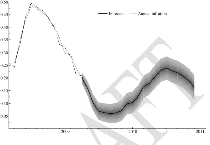
Figure 1 depicts the forecast for Case 1, the worst case, together with two times the
standard error, where we have forecasted annual inflation growth to facilitate interpretation. The
fan chart shows the range of uncertainty indicated by the shaded area around the central
projection. Initially, inflation will continue falling down to about 5 percent, but it then rises
during the drought. The reason for the rapid decline during 2009 is that world food prices are
constant, and domestic prices are high due to recent past and current high inflation. As a result,
the real exchange rate is appreciates in spite of the depreciation of the nominal exchange rate. In
other words, the disequilibrium in the external sector reduces inflation through the error
correction term. The forecast thus illustrates how international market integration keeps domestic
latter half of 2009 and raises inflation to over 20 percent. Of course, these results hinges on the
assumed depreciation of the exchange rate, if the value of the Birr were to fall much more,
possibly due to shortages of foreign reserves, inflation could actually increase.
It is worth emphasizing that although inflation growth declines, it is still positive and
high, and the consumer price level keeps rising. Moreover, the model does not imply that
domestic food prices eventually will decline, even if world food prices fall since the exchange
rate can depreciate, nor does it show that domestic prices eventually will be equal to import parity
prices, since the long-run relationship is an index set to unity in 2006:12.
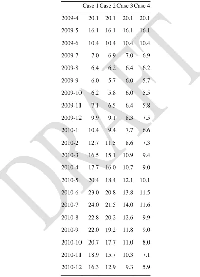
Figure 12 shows the expected developments for annual inflation for all the four cases.
Because of the high past inflation and stable world prices, domestic prices adjust towards long
run equilibrium in all four scenarios during 2009. Case 2 illustrates the role of the exchange rate,
limiting the depreciation to 10 percent makes inflation increase less. In the third case, there is a
good harvest and 20 percent depreciation. As expected, inflation rises a lot less than in the
previous cases, peaking at 14 percent. In the final case, a good harvest and and relatively stabke
exchange rate, keep inflation at single-digit levels most of the time.
Although highly tentative, our four scenarios show the following. First, annual inflation
growth in Ethiopia is likely to decrease over the coming years. This is mainly because of the
strong effect of international food prices on domestic inflation. Yet, annual inflation growth is
still positive, so the level of the overall consumer price index will continue to increase. Moreover,
it is also important to mention that if international prices would start increasing again, they would
Figure 11: Predicted CPI inflation growth for Case 1, 2009:4-2010:12 (annual log growth rates)
2009 2010 2011
0.05 0.10 0.15 0.20 0.25 0.30 0.35 0.40 0.45 0.50
Forecasts Annual inflation
Second, inflation inertia prevents a rapid stabilization of inflation even in very good
circumstances. This is because past inflation to some extent carries over to current inflation, so it
takes several months for a one-time decrease in inflation to have its full impact.
Third, under the presented assumptions, the findings suggest that one of the main driving
forces behind domestic inflation is agricultural output growth. While exchange rate and monetary
policies can make a significant difference, it is crucial to take into consideration the development
of the agricultural economy, in particular the cereal market. Our findings thus suggest that
successful policies should consider supporting both exchange rate stabilization, controlling
money supply growth, and most importantly, boosting and stabilizing domestic food supply. It is
important to mention, however, that the framework presented here is for illustrative purposes
only, as it is based on relationships observed in historical and highly aggregated data, which
should be ideally supported by microeconomic evidence, to draw stronger conclusions.
Moreover, a more complete macro-model would have incorporated the balance of payments and
Figure 12: Illustrative forecast scenarios, 2009:4-2010:12 (annual growth grates in percent)
2008 2009 2010 2011
10 15 20 25 30 35 40 45 50
Annual inflation
Case 1 Case 3
APPENDIX
Table A1: Four Inflation Scenarios
Case 1 Case 2 Case 3 Case 4
2009-4 20.1 20.1 20.1 20.1
2009-5 16.1 16.1 16.1 16.1
2009-6 10.4 10.4 10.4 10.4
2009-7 7.0 6.9 7.0 6.9
2009-8 6.4 6.2 6.4 6.2
2009-9 6.0 5.7 6.0 5.7
2009-10 6.2 5.8 6.0 5.5
2009-11 7.1 6.5 6.4 5.8
2009-12 9.9 9.1 8.3 7.5
2010-1 10.4 9.4 7.7 6.6
2010-2 12.7 11.5 8.6 7.3
2010-3 16.5 15.1 10.9 9.4
2010-4 17.7 16.0 10.7 9.0
2010-5 20.4 18.4 12.1 10.1
2010-6 23.0 20.8 13.8 11.5
2010-7 24.0 21.5 14.0 11.6
2010-8 22.8 20.2 12.6 9.9
2010-9 22.0 19.2 11.8 9.0
2010-10 20.7 17.7 11.0 8.0
2010-11 18.9 15.7 10.3 7.1