Pattern recognition and subjective belief
learning in repeated mixed strategy
games
Spiliopoulos, Leonidas
University of Sydney
10 July 2009
MIXED STRATEGY GAMES
Leonidas Spiliopoulos2,3
Abstract
This paper aspires to fill a conspicuous gap in the existing literature on learning in games, namely the absence of any empirical verification of learning rules involving pattern recognition. An extension of weighted fictitious play is proposed both obeying cognitive laws of subjective perception, and allowing for two-period pattern detection of opponents’ behavior. The unconditional prior probability of a subject employing a pattern detecting belief model is 0.34, as estimated by a mixture (latent-class) model of the elicited belief and action data series fromNyarko and Schotter(2002), or 0.551 using only action data. The conditional prior probability of using pattern recognition was found to depend positively on a measure of the exploitable two-period patterns in an opponent’s action choices, in stark contrast to the minimax hypothesis. Also, standard weighted fictitious play models are found to significantly bias memory parameter estimates upwards, compared to the proposed subjective fictitious play models. Finally, simulations of learning models reveal that the simple win-stay/lose-shift heuristic may be effective even against more complex pattern detecting models.
Keywords:Behavioral game theory; Learning; Fictitious play; Pattern detection; Simulations; Beliefs; Repeated games; Mixed Strategy Nash equilibria; Economics and psychology; Agent based computational economics.
1. INTRODUCTION
Repeated mixed strategy games have been one of the foci of both the experimental game theory literature and its theoretical counterpart -Camerer(2003) andKagel and Roth(1995) are excellent introductions to the field of behavioral and experimental game theory. The literature is rife with experimental studies investigating whether human play is well described by theoretical solutions such as the mixed strategy Nash equilibrium (MSNE), the Quantal Response Equilibrium (McKelvey and Palfrey,1995), or other equilibrium concepts and refinements4
.
These theoretical solutions implicitly assume instantaneous equilibration, and therefore remain silent on the learning dynamics of the off-equilibrium path. In response to this, researchers resorted to postulating theories of learning originally inspired by the psychology and artificial intelligence literature which already had a strong history of grappling with such issues. Most learning rules employed in the literature are derivatives of two basic models, belief learning (Cheung and Friedman,
1997) and reinforcement learning (Roth and Erev,1995), or a mixture of both as in the EWA model
1
This is the first of three papers towards a PhD degree, conferred by the University of Sydney in May 2008. 2
University of Sydney 3
The author would like to thank Kunal Sengupta for constructive input and thesis supervision, Yaw Nyarko and Andrew Schotter for kindly providing the experimental data, Editor David Levine and three anonymous referees for valuable observations, Ananish Chaudhuri and participants at the First Summer Workshop in Experimental Economics and Social Sciences (ExESS), University of Auckland Business School. This research was made possible by funding provided by the Government Department of Education, Science and Training (Australian Government), the College of Humanities and Social Sciences and the Faculty of Economics and Business at the University of Sydney.
4
Examples of specific papers arePalacios-Huerta (2003), Chiappori et al. (2002), Walker and Wooders(2001),
Binmore et al.(2001), Bloomfield (1994), Brown and Rosenthal (1990), Rapoport and Budescu(1997) andLevitt et al.(2008).
(Camerer and Ho,1999). Weighted fictitious play belief learning, henceforth abbreviated towfp, is the basis of the approach that will be employed in this paper and assumes that players form beliefs about their opponent’s future play by observing the historical frequency of their opponent’s actions. These beliefs are then translated into final actions through the use of a stochastic decision rule.
This study will re-interpret the data from the innovative experiment by Nyarko and Schotter
(2002), which directly elicited players’ beliefs about their opponents’ actions. The main contributions of this paper to the existing literature are:
1. The specification of a pattern-detecting weighted fictitious play model and empirical validation of its use by human subjects.
2. The specification of an extension to wfp that incorporates common psychophysical laws of subjective perception, and its validation as a more accurate model of belief formation. 3. An alternative explanation for the existence of negative individually estimated
responsive-ness/sensitivity parameters in decision rules, a result which is normally ascribed either to anticipatory learning (Selten, 1991) or simply irrational behavior. It will be contended that this could occur due to model misspecification if a non-pattern detecting learning model is used to fit the behavior of a pattern detecting player. The same argument will be put forth to explain the occurrence of negative individually estimated memory parameters in weighted fictitious play belief models.
4. The presentation of a taxonomy of heterogeneity which makes important distinctions between the causes of observed heterogeneity in subjects’ behavior. Between-subjects heterogeneity that is due to innate differences in behavior or ability, and within-subjects heterogeneity that is a consequence of subjects conditioning their behavior on characteristics of their opponent’s action choices.
5. Empirical validation of the existence of significant within-subjects heterogeneity as subjects are more likely to using a pattern-detecting belief model the more their opponents deviate from independently distributed (or serially uncorrelated) actions, as prescribed by a mixed strategy Nash equilibrium.
6. Investigation through agent based simulations of the evolutionary fitness of various types of belief learning rules, with and without pattern recognition. The win-stay/lose-shift heuris-tic, despite its simplicity, will be shown to perform very well against more complex pattern detecting models of behavior.
The layout of this paper is as follows. Section2is a literature review drawing both from the behavioral game theory literature as well as from the psychology literature with regards to human ability at randomizing and detecting sequential patterns. Section 3 proposes modifying the parametric form of standard wfp models to allow for pattern detection, and to obey principles of psychophysics and subjective perception. Section 4 presents a taxonomy of heterogeneity and is followed by Section
5 that introduces the original experiment by Nyarko and Schotter (2002). Section 6 presents the results of the estimation of stated belief models using only the elicited beliefs, whereas Section 7
in methodology as agent based computational models are used to evaluate the evolutionary fitness of various belief learning models. Finally, Section10summarizes the main conclusions of this paper.
2. LITERATURE REVIEW
The majority of experimental game theory studies collect data on the observable actions of players and then attempt to fit a model of off-equilibrium behavior. This entails the simultaneous estimation of both the belief generating mechanism, which is not directly observable, as well as the decision rule. Salmon (2001) finds that simultaneous estimation, and therefore indirect estimation of the belief model, often performs poorly in recovering true underlying parameter values. Nyarko and Schotter(2002) made an important contribution to the literature by implementing an experimental setup that made beliefs observable, thereby effectively avoiding the econometric problems of joint estimation. In their paper, they not only collect data on the actions of players in a repeated game with a unique mixed strategy Nash equilibrium (MSNE), but also elicit beliefs by asking players to state the probability with which they thought their opponents would play their pure strategies before each round.
There exist very few theoretical studies of learning models incorporating pattern recognition in the game theory literature, and to the best of our knowledge, no relevant empirical studies.Fudenberg and Levine (1998) in their authoritative book on learning in games discuss some of the theoretical implications of what they refer to as conditional fictitious play. This is defined as a broad class of fictitious play learning algorithms where fictitious play frequencies are calculated for each of a number of predefined disjoint subsets of the history of play, instead of the standard case where these frequencies are calculated over a single set of the history. Beliefs are then calculated by conditioning on the last realized subset of play i.e. using the associated fictitious play frequencies corresponding to that particular subset. A special case of this broad range of learning rules will be employed in this paper, with the subsets of the history defined as the strategies consisting of all two-period temporally consecutive combinations of an opponent’s actions.
Aoyagi (1996) proves that in zero-sum games with a unique Nash equilibrium, if both players follow conditional fictitious play rules that asymptotically recognize patterns of the same length, then players’ beliefs converge to the Nash equilibrium action profile with probability one. Sonsino
(1997) examines the convergence properties of game play when players can recognize cyclical strategic patterns in opponents’ behavior, proving that convergence to fixed patterns of pure strategy Nash equilibria occurs with probability one for a large class of games. Finally, it was proven that a necessary condition for convergence to a mixed strategy Nash equilibrium is the use of arbitrarily long histories of play.
2.1. Literature review of humans’ (in)ability to randomize
emulating.
Game theorists have been interested in these documented inefficiencies of human randomization as they imply that one should expect deviations from the MSNE prescription of independently distributed actions. Palacios-Huerta (2003) and Chiappori et al. (2002) investigate penalty kicks in professional soccer, concluding that the minimax hypothesis cannot be rejected.Palacios-Huerta and Volij(2008) find that professional soccer players exhibited transfer of learning as they continued to play according to minimax even in laboratory settings. On the other hand, Levitt et al. (2008) compare college students and professional soccer, bridge, poker players in laboratory settings, finding significant deviations from MSNE behavior for all groups indicating that the professional players have not transferred their learning from the field.Walker and Wooders(2001) examine tennis serves and find that there is evidence of professional players conditioning on past actions, but behavior is closer to the MSNE for professional players or experts than for inexperienced subjects.
In conclusion, the verdict is still out with regards professionals playing the MSNE when outside of their field of expertise. However, the literature is more consistent in its findings that non-professionals that do not have a long history of playing a specific game with large enough monetary incentives to fine-tune their strategies will not conform closely to the MSNE prescription of serially uncorrelated action choices.
2.2. Literature review of pattern detection or sequence learning in humans
The question of whether humans have the ability to detect patterns is a well established research topic in the psychology literature referred to as sequence learning, Clegg et al. (1998) provides a concise introduction. Explicit learning is the result of conscious and intentional cognitive processes that subjects are able to report, whereas implicit learning occurs subconsciously rendering the subject unaware and therefore unable to directly acknowledge this type of learning (Cleeremans et al.,1998). The seminal paper by Nissen and Bullemer (1987) advanced the view that sequence learning is primarily an implicit, rather than explicit, form of learning. The current state of the literature has accepted that humans engage in sequence learning and the latest research is primarily directed at using different experimental methodologies to indirectly reveal implicit learning, with the purpose of determining the relative importance of explicit versus implicit learning.
Before proceeding further it is necessary to define sequence learning and a measure of the depth of such learning. The definition of nth order probability information is the use of information at time t−n+ 1 to infer behavior at time t. If information from all periods between t−n+ 1 and
t−1are used then this is referred to asnth order adjacent dependency, alternatively if not all of the periods are relevant then it is referred to as non-adjacent dependency5
. Sequence learning involves pattern detection because adjacentnth order probability information essentially involves recognizing
nconsecutive time period strategies or patterns. For example, second-order probability information involves calculating the probability of an action conditional on the action played in the previous
5
period.
The existence of sequence learning is well documented by studies such as Remillard (2007) and
Remillard and Clark(2001), who find evidence of implicit sequence learning of second- through to fifth-order adjacent and non-adjacent probabilities. Other studies in the experimental psychology field, such asGomez(1997), have found evidence of explicit knowledge of second-order probabilities in which the subjects were consciously aware of their learning. Whether sequence learning is pre-dominantly implicit or explicit has important implications for experimental game theoretic models of pattern recognition. If such learning is explicit then it should be detectable in the elicited belief series, whereas if it is implicit then its effect would only be indirectly apparent when using action data to estimate the learning models.
In conclusion, the aforementioned research justifies investigating pattern recognition models of learning in game theory as they have documented that pattern detection of sufficient depth is possible in the human brain, both explicitly and implicitly.
3. PROPOSED EXTENSIONS TO STANDARD WEIGHTED FICTITIOUS PLAY
This section will propose two significant extensions of the standard weighted fictitious play model used in the literature. The first extension will directly model pattern recognition in the belief for-mation process. The second extension, referred to as subjective fictitious play, sfp henceforth, will incorporate common principles of subjective perception, whilst also nesting the standardwfp model for specific parameter values. Finally, the consequences of allowing negative estimates of key param-eters will be discussed, in particular how this may allow non-pattern detecting learning models to indirectly capture two-period patterns.
3.1. Modification of learning rules to include cases of pattern recognition
In standard weighted fictitious play (Cheung and Friedman, 1997), or equivalently single-period fictitious playfp1,the beliefs,fp1i,t(aj), of playeriregarding the probability of his opponent playing
actionaj are equal to the countCi,t(aj), presented in equation 1. Letai represent the action taken
by playeriand for any actionaj, define playeri’s count ofaj at timet≥2 as:
(1) Ci,t(aj) =
It−1(aj) +!tu−2=1γiu·It−u−1(aj)
1 +!tu−2=1γu i
The indicator functionIt(aj), takes the value of one if playerj chose actionaj in time periodt or
the value of zero otherwise. The memory decay parameter for each player is γi and memory loss
from the MSNE predictions of observed frequencies of single period actions6
.
The fp1 algorithm however is not designed to detect second- and higher-order deviations from the MSNE because it does not keep track of consecutive temporal sequences of actions. Fictitious play can be generalized to what shall be referred to as n-period (weighted) fictitious play (fpn) wherenis an integer greater than or equal to one and refers to the complexity and depth of pattern detection7
. Fp2 is more sophisticated than fp1 because it tracks how many times two temporally consecutive sequences of actions have been observed and then conditions the probability of an action being played on the previous action chosen by the opponent. In this case it is assumed that a player is making use of second-order probability information8
. For example, suppose our opponent’s play is r-r-g-g-r-r-r9
, fp2 will evaluate how often the following sequences have turned up in past play: r followed by r, g followed by g, r followed by g and g followed by r.
Let the subscriptsiand j denote two different players, then given actionsaj anda′j, It(aj|a′j)is
an indicator function that takes a value of one ifaj was the action played at timetanda′j was the
action played at timet−1and a value of zero otherwise. Define for playeriat timet≥3, the count ofaj given actiona′j with memory parameterγi as:
(2) Ci,t(aj|a′j) =
It−1(aj|a′j) +
!t−2
u=1γiu·It−u−1(aj|a′j)
1 +!tu−=12γu i
Thefp2 beliefs of playeriregarding actionaj given actiona′j from the discrete strategy setSj of
playerj is10
:
(3) fp2i,t(aj|a′j) =
Ci,t(aj|a′j)
!
aj∈SjCi,t(aj|a
′
j)
Subjects’ decisions as to what depth of pattern recognition to employ will depend not only on the likely depth of an opponent’s behavioral patterns but also on the cost of detecting these patterns. The number of frequency variables or counts anfpnbelief model must keep track of is the number of actions available raised to the power ofn. Also, further cognitive resources are needed to remember the last n−1 periods of play in order to be able to condition, so that the cognitive requirements increase withnat a faster than exponential rate. Increasing the size of the action space or the depth of pattern recognition leads to drastically higher computational cost and therefore pattern detection
6
Shachat and Swarthout(2004) empirically verify that humans better respond to deviations in first-order proba-bilities of play as long as they are relatively far away from the MSNE.
7
This proposed learning rule is a special case of the class of learning rules thatFudenberg and Levine(1998) refer to as conditional fictitious play.
8
In general anyfpnmodel usesnth order adjacent probability information. 9
Counts are created by allowing for overlapping sequences so that each action is counted twice, once as the last action in one 2-period sequence and one as the first action in another 2-period sequence. This is because there is an inherent problem in that two very different sequences can be obtained by changing when the counting starts. Also if overlapping sequences are not used then conditioning on the previous action will be problematic.
10
This definition assumes that the denominator is not zero i.e. that the actiona′
j has been played at least once
in the past. In cases wherea′
will likely be restricted to relatively low depth.
3.2. On a subjective variant of weighted fictitious play incorporating psychophysical principles of perception
Aside from introducing a pattern detecting variant of weighted fictitious play, this paper ad-vances the existing literature by allowing players’ perceptions to follow commonly ascribed rules of psychophysics pertaining to the translation of physical, or objective, stimuli to their subjective corre-lates in the human mind. Specifically, equation4presents the class of belief learning rules henceforth referred to as subjective fictitious play, denoted by sfpni,j,t (of order n, at timet, for individuali
and action j - the latter subscript will henceforth be dropped for simplicity). The encapsulating non-linear function in equation4 transforms the objective fpn variables presented above to player
i’s final subjective beliefs.
(4) sfpni,t =
δi(fpni,t)λi
δi(fpni,t)λi+ (1−fpni,t)λi
This specific functional form has been used in the choice under uncertainty literature (Goldstein and Einhorn,1987;Kilka and Weber,2001;Lattimore et al.,1995) as a behavioral model of proba-bility weighting functions, transforming objective probabilities to subjective probabilities. It exhibits the following two desirable properties and advantages over standardwfp.
Firstly, it incorporates principles of subjective perception since the curvature of the function is controlled by the discriminability parameterλi, allowing the subjective sensitivity tofpni,t to vary
over its domain. Conveniently, ifλi= 1a simple linear relationship ensues implying that subjective
beliefs are equivalent to objective beliefs. For values of 0 < λi < 1 the function is concave over
domain values from zero to some critical value less than one, and convex thereafter till a value of one. Alternatively, if λi > 1 this is reversed as the function changes from convex to concave.
The attractiveness parameter,δi controls the elevation of the function thereby allowing for a prior
inclination in beliefs that an opponent is more likely to play certain actions than others. For example, a player may exhibit such an inclination based on the payoff structure of the game.
Secondly, this parametric form nests many other important models, in particular the constraints
λi=δi = 1reduce the model to the standard weighted fictitious play modelsfp1 andfp2.Another
important baseline model is constant beliefs with random fluctuations, which is captured by this model whenλi= 0, with the mean of the stated beliefs controlled by parameterδi.
3.3. Stochastic decision rules
Players are assumed to stochastically best respond to the expected payoffs of actions given their beliefs. The decision rule in equation5defines the probability of subjectiplaying actionai,P ri,t(ai),
as a logit function where Si is the discrete strategy set of player i, and E(π(ai)) is equal to the
expected payoffs of playing action ai given beliefs over all the opponent’s actions aj ∈ Sj. The
and is assumed to be the same for all actions. As βi →0 the probability distribution over actions
tends to the uniform distribution where all actions are played with equal probability. However, as
βi → ∞the decision rule approaches deterministic best response, where the action with the highest
expected payoff will be played with certainty. Finally, players’ action choices may be affected by a judgment that is independent of the evolution of play, captured by the constant αai, which is
different for each actionai.
(5) P ri,t(ai) =
eαai+βi·E(π(ai))
!
ai∈Sie
αai+βi·E(π(ai))
3.4. Indirect detection of patterns by unrestricted non-pattern detecting belief models
Despite the expectation that the memory parameter in a belief model should be positive, previous studies have not imposed this on the econometric models, and in many cases individual estimates are found to be less than zero (Cheung and Friedman,1997;Nyarko and Schotter,2002). However, as will be elaborated below, negativeγivalues in conjunction with a non-pattern detecting fictitious
play belief model may be capable of indirectly capturing patterns.
Assume that there exists negative serial correlation in an opponent’s action data so that actions alternate more often than would be expected with independent draws. This will necessarily lead to negatively correlated fictitious play beliefs regardless of the sign ofγi, however whether these beliefs
are in phase with the patterns will depend on the sign. Ifγi >0 the fictitious play beliefs at time t for the action played at time t−1 will be higher than the beliefs at t−1. This result is clearly inconsistent with the negative correlation in the action sequence, and therefore pattern recognition is impossible as the belief model will on average be predicting the wrong action. However, ifγi <0,
the opposite will hold so that the fictitious play beliefs are moving in the correct direction as if they were anticipating the negative correlation in actions.
Givenγi<0then a decision rule will best respond to the patterns if the expected payoff difference
between the two actions alternates on either side of zero. One way of accomplishing this is to ensure that for consecutive rounds beliefs alternate in different regions of the best response probability space i.e. if the MSNE is to play an action with probability 0.6, the beliefs will have to alternate on either side of 0.6. This can always be accomplished by anfp1 model by settingγito be negative and
arbitrarily close to zero, as a reduction in memory depth increases the variability of fitted beliefs ultimately leading them to be arbitrarily close to 0 and 1. Econometric estimation ofsfp1 can also accomplish this another way as there necessarily exists a value ofδthat will guarantee this behavior. Similarly, this requirement could be achieved directly by the decision rule through the manipulation ofα. Hence, misspecification due to the modeling of a pattern detecting subject with a non-pattern detecting belief model could lead to identification problems for these three parameters as they are all associated with indirectly capturing patterns. Given that previous studies employed standard non-pattern detecting fictitious play models, it is possible that the negative estimates of individual memory parameters are a result of this misspecification.
Figure 1.— A taxonomy of heterogeneity
heterogeneity
within-subjects (conditional)
between-subjects (unconditional)
extrinsic intrinsic within-rule between-rule
econometric models, even though in the absence of anticipatory learning (Selten, 1991) this is a reasonable conjecture. Although anticipatory learning is certainly a possibility, it requires extreme sophistication on behalf of experimental subjects, whereas there exists a much simpler explanation. A non-pattern detecting model, whether it befp1 orsfp1, is still capable of best responding to two-period patterns in an opponents’ action sequence when γi >0 ifβi <0. The argument is identical
to that just made above, replacing γi with βi. Therefore it is likely that the negative estimates
of individual sensitivity/responsiveness parameters of prior studies are indirectly capturing pattern detection on behalf of subjects.
In order to avoid these issues which would blur the distinction between pattern detecting and non-pattern detecting models, all estimated models in this paper will restrictγˆi andβˆi to be necessarily
non-negative.
4. ON A TAXONOMY OF HETEROGENEITY
Despite the empirical confirmation of subject heterogeneity in experimental games, analysis is pursued without regards to the different possible sources of heterogeneity in subjects’ behavior. This paper will proceed in defining a taxonomy of heterogeneity and providing empirical evidence of the relative importance of the various taxa. It will become clear in the ensuing discussion that identifying the sources and types of heterogeneity exhibited by subjects is of paramount importance in truly understanding strategic decision making.
each player chose to employ a different learning rule by conditioning on some information. Between-subjects (unconditional) heterogeneity is defined as the heterogeneity that arises if the observed learning rules were not elements in the sets of all the players so that the observed heterogeneity occurred not due to choice but due to an inherent inability i.e. cognitive bounds that differ amongst subjects. With regards to this study between-subjects heterogeneity assumes that not all subjects are privy to the pattern detecting model sfp2, perhaps due to different cognitive bounds. Within-subjects heterogeneity, on the other hand, implies that each player has the ability to use the sfp1
and sfp2 learning models but chooses which learning rule to employ by observing whether their opponent exhibits serially correlated behavior. If not, then a player may employ thesfp1 rule which has lower computational costs, otherwise the player may switch to thesfp2 rule instead.
Spiliopoulos (2008) specifically designed an experiment to discriminate within- and between-subjects heterogeneity by observing how each subject behaved against three different predetermined computer algorithm opponents. Within-subjects heterogeneity was found to be a significantly more important source of behavioral heterogeneity than between-subjects, demonstrating the necessity of acknowledging this in behavioral modeling.
Having defined the first hierarchical level of taxa, within-subjects heterogeneity can be further subdivided into two further taxa, coined as extrinsic and intrinsic within-subjects heterogeneity. The latter refers to heterogeneity that is conditioned on variables pertaining to game play, essentially referring to whether subjects adapt their strategy to the opportunities for exploitation presented by their opponent. Extrinsic within-subjects heterogeneity is essentially heterogeneity that cannot be attributed to the game play variables that a researcher would include in an econometric model, and therefore would be captured in the error term. Note, that this taxa includes both the cases where subjects may be conditioning on extrinsic but theoretically observable random variables i.e. sunspots, and the effects of extrinsic but non-observable variables such as the levels of various neurotransmitters in the brain and how they affect behavior.
Finally, for the purposes of this study we will distinguish between two other taxa of between-subjects heterogeneity: between between-subjects, within-rules and between-between-subjects, between-rules hetero-geneity. The latter refers to the availability of different learning rule models, in this casesfp1 and
sfp2. The former refers to heterogeneity in the parameter estimates of rules that are available to players, as is the case if two subjects both use thesfp2 rule, but the estimatedsfp2 model for both of them exhibits significantly different parameter values.
5. DATASET AND METHODOLOGY
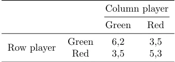
The N&S game is given in TableI, and the experimental data used was the treatment where each subject repeatedly playing the same game 60 times against the same opponent. The mixed strategy Nash equilibrium for both players was to play red 60% of the time and green 40%. Subjects would receive monetary compensation both according to their payoffs from playing the game and from the accuracy of their stated beliefs compared to opponents’ realized actions11
.
Three different approaches will be employed to obtain the necessary empirical results. Section6will directly estimate models of subjects’ elicited beliefs without resorting to their action choices. Section
11
TABLE I N&S Payoff matrix
Column player
Green Red
Row player Green 6,2 3,5
Red 3,5 5,3
7 will model subjects’ action choices using a two-stage procedure where the fitted belief estimates from the previous section are used as regressors and the decision rule parameters are estimated using a concomitant, mixed effects, latent class logit regression. Section8will simultaneously estimate both the underlying belief formation model and the decision rule using subjects’ action data, without utilizing the elicited belief series. Finally, Section 9 will simulate play based on the interactions of different types of learning rules and parameter values in order to ascertain their evolutionary fitness.
6. ESTIMATION OF STATED BELIEF MODELS
Four different equations will be estimated using the competing belief models fp1, fp2, sfp1 and
sfp2.The estimation problem at timetis represented by equation6, wheresbi,tis equal to playeri’s
stated belief regarding actionj andsfpni,t (or alternatively fpni,t) is the fitted belief. To allow for
beliefs to settle, in particular for thefp2 andsfp2 models which require a longer initial history to form beliefs regarding all possible two-period combinations, the first ten rounds are not included in the measure of fit, however these values are used in the formation of beliefs. Optimization is performed in two steps, first a randomly generated population of parameter estimates is subjected to a genetic algorithm, and the best candidate is used as a starting point for a quasi-Newton Sequential Quadratic Programming algorithm, implemented in Matlab as thefmincon function.
(6) min
γi,δi,λi
60
"
t=11
[sbi,t−sfpni,t]2 0≤γi≤1, δi≥0, λi≥0
Comparisons between different belief models and their performance will be exacted by 10-fold cross-validation. The dataset is divided into ten non-overlapping folds of five rounds, and the models are estimated each time by training on nine of the folds and measuring the out of sample error performance on the remaining fold. The cross-validation MSE allows comparisons amongst models with different degrees of freedom, as it bypasses the problem of overfitting to the training data. Tables
IIandIIIpresent the results of the optimization of the class of models represented by equation 6.
6.1. Do the subjective belief models, sfp1 and sfp2, predict stated beliefs more accurately than the standard or objective fictitious play models?
TABLE II
Mean square error (MSE) of individually estimated models
In sample 10-fold CV
Player fp1 fp2 sfp1 sfp2 fp1 fp2 sfp1 sfp2
1 0.062 0.102 0.038 0.077 0.063 0.103 0.046 0.087 2 0.020 0.026 0.011 0.011 0.020 0.026 0.011 0.011 3 0.143 0.135 0.141 0.131 0.148 0.140 0.152 0.154 4 0.061 0.107 0.051 0.049 0.061 0.111 0.054 0.054 5 0.162 0.028 0.139 0.024 0.163 0.029 0.141 0.024 6 0.125 0.135 0.106 0.105 0.133 0.136 0.118 0.117 7 0.081 0.080 0.036 0.036 0.111 0.091 0.042 0.044 8 0.063 0.065 0.051 0.052 0.063 0.064 0.058 0.064 9 0.047 0.042 0.030 0.021 0.051 0.044 0.032 0.023 10 0.087 0.116 0.069 0.069 0.091 0.118 0.073 0.087 11 0.225 0.004 0.217 0.003 0.225 0.005 0.220 0.007 12 0.102 0.104 0.078 0.080 0.102 0.104 0.084 0.090 13 0.026 0.028 0.024 0.023 0.026 0.028 0.025 0.024 14 0.029 0.034 0.027 0.026 0.029 0.034 0.033 0.029 15 0.086 0.089 0.086 0.086 0.088 0.089 0.095 0.093 16 0.130 0.162 0.099 0.099 0.129 0.163 0.105 0.103 17 0.171 0.169 0.138 0.157 0.200 0.169 0.146 0.189 18 0.059 0.055 0.057 0.055 0.059 0.055 0.059 0.063 19 0.008 0.016 0.004 0.006 0.008 0.016 0.005 0.007 20 0.020 0.031 0.019 0.020 0.020 0.031 0.021 0.021 21 0.039 0.044 0.012 0.012 0.039 0.044 0.013 0.014 22 0.077 0.090 0.065 0.085 0.079 0.090 0.067 0.096 23 0.016 0.014 0.011 0.009 0.016 0.014 0.012 0.010 24 0.051 0.061 0.033 0.045 0.055 0.063 0.035 0.056 25 0.061 0.061 0.045 0.045 0.061 0.061 0.051 0.050 26 0.071 0.077 0.069 0.072 0.080 0.077 0.081 0.080 27 0.219 0.228 0.181 0.182 0.219 0.229 0.194 0.195 28 0.158 0.164 0.120 0.148 0.174 0.166 0.161 0.179
Average 0.086 0.081 0.070 0.062 0.090 0.082 0.076 0.070
is strongly rejected(z= 2.701, p= 0.0069), likewise when comparing fp2 andsfp2 (z= 2.803, p= 0.0051). These two results provide significant evidence that beliefs are not modeled accurately by the standard fictitious play functional form, and fitting beliefs to these models may lead to significant misspecification bias in the estimates of parameters, especially for γ as will be argued in the next section.
6.2. Estimates of the memory parameter,γˆ
Estimates of the memory parameters from the standardwfp models in N&S were centered on one with little dispersion, implying that individuals weighted all past information equally. However, as they point out this is likely the result of the restriction of a one parameterwfp model in estimating a highly variable stated belief series. The best such a model can accomplish is to approximately fit the mean of the elicited belief series with a relatively smooth, stable empirical data series. This can only be accomplished by a high value ofγˆ which minimizes the variability in the empirical beliefs series. However, the subjective belief models can be calibrated to the mean of the stated beliefs by controlling the elevation of the subjective beliefs through the δparameter, thereby alleviating this possible misspecification problem. The strong evidence for the subjective belief models supports the contention that the standard wfp model is indeed misspecified and therefore parameter estimates may be biased.
The results presented in Table III verify this intuition as ˆγ falls from 0.950 to 0.501 for thefp1
and sfp1 models respectively, and from 0.937 to 0.814 for fp2 and sfp2 respectively. Hence, the finding of memory parameter estimates near a value of one for fp1 belief models is most likely due to the inherent model misspecification in standard fictitious play models which does not permit the calibration of the elevation of stated beliefs. Finally, a two-tailed sign test strongly rejects the null hypothesis(p= 0.002)that the median of the paired differences in estimates ofγˆfromsfp1 andsfp2
for each player is equal to zero. The significantly higher value of ˆγ for pattern detecting models is reasonable as greater memory depth is required to effectively detect patterns in opponents’ behavior. Another interesting observation is thatˆγfor thesfp1 models in often equal to or close to zero, in particularγ <ˆ 0.1 in 10 cases. Hence, the sfp1 model is often capturing a special case of weighted fictitious play behavior, namely Cournot beliefs. Note that only in two cases is γ <ˆ 0.1 in the estimated sfp2 models, in concurrence with the assumption that pattern detecting models should exhibit high memory parameters.
6.3. Estimates of the discriminability coefficient,λˆ
The mean estimates of the discriminability coefficient forsfp1 andsfp2 respectively are 0.581 and 0.42612
(or excluding zero estimates 0.74 and 0.477 respectively), so that for most players beliefs are concave for values of thefpnvariables between zero and an interior inflection point, and convex thereafter. These results are in accord with common principles of psychophysics as small deviations from the MSNE should be less likely to be detected than large deviations. Also, larger deviations are more likely to be due to true deviations in the underlying data generating process rather than noise and therefore players should be more likely to respond to larger deviations.
6.4. Estimates of the attractiveness coefficient, ˆδ
The elevation of the subjective function is controlled by the estimate ofδˆ, with mean estimates forsfp1 andsfp2, 0.995 and 1.037 respectively. A null hypothesis that the median of the distribution
12
TABLE III
Comparison of parameter estimates of individually estimatedfpn andsfpn models
fp1 fp2 sfp1 sfp2
Pl. γˆ γˆ γˆ δˆ λˆ γˆ δˆ λˆ
1 0.756 0.000 0.897 0.954 3.423 0.641 2.368 0.109
2 1.000 1.000 - 0.894 0.000 - 0.894 0.000
3 0.885 0.957 0.896 0.825 1.160 0.877 0.910 0.522
4 1.000 1.000 - 0.773 0.000 - 0.886 0.000
5 0.953 0.835 - 0.938 0.000 0.996 0.241 0.869 6 0.955 0.999 1.000 0.847 0.127 1.000 0.791 0.031 7 0.869 0.922 0.070 0.690 0.066 0.767 0.610 0.413 8 1.000 1.000 0.017 1.133 0.026 0.856 1.103 0.151 9 0.985 0.885 0.036 1.075 0.056 0.739 1.085 0.322 10 0.923 0.932 0.922 0.508 0.189 0.009 0.521 0.007 11 1.000 0.786 - 1.023 0.000 1.000 0.324 2.304 12 1.000 1.000 0.719 1.322 0.211 1.000 1.279 0.275 13 1.000 1.000 0.031 0.939 0.015 1.000 0.987 0.304 14 1.000 1.000 1.000 1.385 0.245 1.000 1.336 0.251 15 0.997 1.000 0.005 0.840 0.016 1.000 0.853 0.342 16 1.000 0.969 1.000 0.541 0.790 0.956 0.635 0.242 17 0.516 1.000 0.003 0.750 0.055 1.000 0.669 0.920 18 1.000 1.000 - 1.070 0.000 1.000 1.000 0.749 19 1.000 0.997 0.016 1.072 0.020 0.573 1.097 0.021 20 1.000 0.998 0.042 1.003 0.020 0.790 1.014 0.032 21 1.000 1.000 0.006 0.903 0.003 0.271 0.914 0.004 22 1.000 1.000 0.044 2.000 0.096 0.995 2.447 0.329 23 1.000 1.000 0.696 1.033 0.136 0.833 1.088 0.270 24 0.933 0.958 0.852 1.036 0.236 - 1.075 0.000 25 0.985 1.000 - 0.982 0.000 0.050 0.977 0.006 26 0.845 1.000 0.782 0.957 0.624 1.000 0.796 0.840 27 1.000 1.000 0.998 2.354 1.225 1.000 2.892 0.490 28 1.000 1.000 1.000 0.006 7.529 1.000 0.256 2.126
TABLE IV
Pooled estimation ofsfp1 andsfp2 models
In sample MSE Cross-validation MSE γˆ δˆ λˆ
sfp1 0.0837 0.0839 1 0.999 0.428
sfp2 0.0780 0.0782 0.682 1.063 0.112
of individual estimates is equal to one can not be rejected in both cases by two-sided sign tests,
p = 0.572 and p = 0.442 respectively. Although the medians are not significantly different from the value ofδ implied by the standardfpn models, this does not exclude the possibility that there exists considerable subject heterogeneity in the individual estimates that must be modeled using
sfpn models rather than the standard objective belief models. The large dispersion of estimates indicates that a significant part of the variance is indeed due to heterogeneity and not just imprecise estimates.
6.5. Does there exist significant between-subjects, within-rules heterogeneity in parameter estimates of the sfpn models?
Pooling the estimation of sfp1 and sfp2 models leads to significantly worse cross-validation per-formance as documented in Table IV. In particular, CV-MSE worsens from 0.076 to 0.0837 for
sfp1 (z = 2.395, p = 0.0166), and from 0.07 to 0.078 for the sfp2 model (z = 2.701, p = 0.0069), both results highly significant according to Wilcoxon signed-rank tests performed on the ten paired cross-validation observations. Misspecifying the models by assuming player homogeneity and pooling subjects leads to estimated values of ˆγ andˆλthat are very different from the majority of the indi-vidually estimated parameters presented in the previous sections. This is in accord withCabrales and Garcia-Fontes (2000) who simulate the econometric properties of learning model estimation, concluding that ignoring subject heterogeneity can seriously bias parameter estimates.
7. TWO-STAGE ESTIMATION OF BELIEFS AND DECISION RULES
This section proceeds with analyses of subjects’ behavior based on both the action data and the elicited belief series. The first stage is the estimation of the individual belief model parameters as executed in the previous section by fitting directly to elicited beliefs, whilst the second stage will estimate the remaining decision rule parameters by simulated maximum likelihood.
Model 1 is a latent class, mixed effects, concomitant discrete choice model represented by equations
7-10, and nests all the other models that will be estimated as special cases.
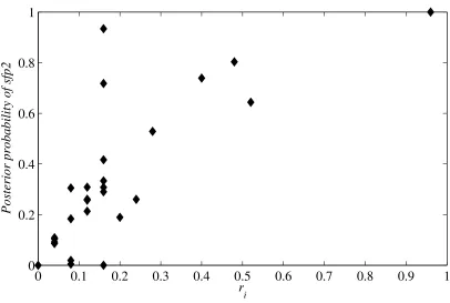
Latent class or mixture models assign a prior probability that each subject belongs to a particular class, in this case whether they are using ansfp1 orsfp2 model with prior probabilities denoted by 1−pandp respectively.Concomitant latent class regression models are an extension where prior class probabilities may be influenced by other covariates or concomitant variables. In this model the covariate isri, the absolute percentage difference between the expected number of runs, assuming
prior class probability is given by equation9including the necessary parameter constraints to ensure that both the minimum and maximum lie between zero and one.
The concomitant specification captures within-subjects heterogeneity, allowing for the possibility that players have access to bothsfp1 andsfp2 belief models, but choose which one to use depending on whether an opponent is displaying two-period patterns that could be exploited. Hence, if ψ >
0 this implies that there exists intrinsic within-subjects heterogeneity. The existence of between-subjects heterogeneity can be confirmed if0 < p <1 when ri = 1. Assuming that the existence of
perfectly correlated actions is detected with certainty by all subjects, then any subject capable of usingsfp2 should also do so with certainty, with the caveat that the additional computational cost of pattern recognition is less than the resulting gains. Similarly, ifri= 0the lower computational cost
of sfp1 should ensure13
that it is used with certainty if there does not exist any between-subjects heterogeneity. Finally, the unconditional prior probability of a subject employing thesfp2 belief rule is obtained by integrating outri from the conditional probability and is given byp#=271
!27
i=1p.
A logit link function qt is employed to transform the attractions into probabilities, where the
attraction for the green action is normalized to a value of one, as shown in equation8, andE∆πt(sfpn)
represents the difference in expected payoffs for choosing the green action over the red action at time
taccording to a specific belief model.
Finally, a mixed effects specification was chosen as a solution to the necessity of modeling individual parameter heterogeneity in the decision rule whilst keeping the degrees of freedom at reasonable levels. The decision rule parametersθ= [α, β]are assumed to be jointly normally distributed with full covariance matrix as given in equation10.
All other models that will be estimated will be nested within Model 1, arising from specific parameter restrictions. Model 2 restricts Model 1 by assuming that prior class probabilities do not depend on the variablerii.e. that there exists no within-subjects heterogeneity. Whereas these two
models allow for two classes within the population, models 3 and 4 assume that either all subjects aresfp2 orsfp1 players respectively. Finally, model 1* is identical to model 1 with the exception that fittedfpnbeliefs are used in the place ofsfpnbeliefs to allow an analysis of the possible consequences of this type of misspecification.
Estimation of all models is performed by simulated maximum likelihood with 500 antithetic draws from the multivariate normal distribution for θ using the Cholesky transformation. The first step in optimizing this function was to randomly select a population of parameter estimates and subject them to a genetic algorithm selection process. The best fitting parameter estimates were then used as the starting point for a quasi-Newton Sequential Quadratic Programming optimization technique implemented as the fmincon function in Matlab. Finally, the whole process was repeated 10 times and the resulting best fitting parameters are reported.
13
ll= 27
"
i=1
ln
$%
(1−p) 60
&
t=11
qt(sfp1)at[1−qt(sfp1)]1−at
(7)
+p
60
&
t=11
qt(sfp2)at[1−qt(sfp2)]1−atdθ
'
(8) qt(sfpn) =
(
1 +eα+eβE∆πt(sfpn)
)−1
n= 1,2
(9) p= 1−e−(φ+ψ·ri) φ≥0, φ+ψ≥0
(10) θ= [α, β]∼N
*
[µα, µβ],
+
σα σαβ σαβ σβ
,-Standard errors will be estimated using a jackknife procedure which involves dropping one individ-ual at a time from the training dataset and re-estimating the model parameters. The log-likelihood of the subject excluded from each run llcvi is a cross-validation measure of fit that allows
compar-isons between models with different degrees of freedom. The sum of the individual cross-validation log-likelihoodsllcv, will be used for model comparison, as will the Akaike and Bayesian information
criteria.
The N&S dataset consists of 14 pairs of players, however this analysis will proceed by dropping player 11 on the basis that it is a severe outlier exhibiting particularly perplexing/irrational behavior. Player 11’s opponent exhibits severe negative serial correlation in action choices, leading to easily detectable two-period patterns. Player 11’s elicited beliefs show that he/she has indeed detected the patterns, but instead of playing a best response to these beliefs the action data in every single case is consistent with the worst response. Hence, from the elicited belief series player 11 is clearly employing asfp2 belief model, but estimation using the observable action data concludes that this player uses ansfp1 model. The only plausible explanation for this clearly irrational behavior is that this player may have simply misunderstood the payoff matrix, and have erred in concluding what the best response action is. The extremeness of this internally inconsistent behavior justifies labelling player 11 as an outlier and excluding him/her from the following analysis.
TABLE V
Maximum likelihood action data models
Model 1 2 3 4 1*
Restriction ψ= 0 p= 1 p= 0
#
p 0.337 (0.036) 0.362 (0.045) - - 0.347 (0.047)
µα 0.031 (0.016) 0.042 (0.017) 0.04 (0.015) 0.048 (0.016) 0.064 (0.012) σα 0.609 (0.032) 0.579 (0.028) 0.505 (0.028) 0.55 (0.035) 0.441 (0.029) µβ -0.623 (0.062) -0.499 (0.07) -0.85 (0.059) -0.7 (0.064) -1.1 (0.098) σβ 1.033 (0.041) 0.812 (0.06) 1.09 (0.052) 1.009 (0.058) 0.987 (0.136)
φ 0 (0) 0.449 (0.069) - - 0 (0.049)
ψ 2.685 (0.383) - - - 2.778 (0.637)
ll(df) 853.901 (7) 855.625 (6) 873.519 (5) 888.737 (5) 872.48 (7)
AIC 1721.8 1723.2 1757.0 1787.5 1759
BIC 1758.3 1754.5 1783.1 1813.5 1795.4
llcv 857.89 860.682 876.524 892.486 883.584
7.1. Does the data support the hypothesis of belief model heterogeneity with respect to whether subjects use pattern recognition?
Models 1 and 2 assume the existence of belief model heterogeneity through a mixture specification which allows each subject to use any of the two belief models, whereas models 3 and 4 assume that all players are using the same model. Comparisons of models with a different number of latent classes can not be performed using standard LR tests even though the models are nested, because the null hypothesis exists on the boundary of the parameter space and therefore the ratio of likelihoods does not follow aχ2 distribution (Titterington,1990). The literature instead proposes information criteria tests or cross-validation as a means of selecting the appropriate number of latent classes. Since the AIC, BIC andllcv for models 1 and 2 are lower than those of models 3 and 4, these criteria
conclude that there exists significant heterogeneity that must be modeled by the latent class/mixture approach of models 1 and 2.
7.2. Does the data support the hypothesis of intrinsic within-subjects heterogeneity conditioned on opponents’ deviations from serially uncorrelated action choices?
In the context of this experiment we define within-subjects heterogeneity as arising from condition-ing on the behavior of a player’s opponent, namely the presence of exploitable two-period patterns. The null hypothesis that there exists no within-subjects heterogeneity is tested by comparing models 1 and 2, the latter incorporating the restrictionψ= 0.
Given that the two models are nested, preference is given to nested tests over non-nested, as the former should exhibit more desirable econometric properties. An asymptotic LR test provides strong evidence of within-subjects heterogeneity with significance at p= 0.0634 (χ2 = 3.447). Also, using the jackknife standard error, the 95% confidence interval14
forψis[1.99,3.63]indicating clearly that
ψ is significantly different from zero. Turning to non-nested tests, this conclusion is confirmed as
14
Figure 2.— Posterior probability ofsfp2 versus the degree of exploitable patterns
0
0.1
0.2
0.3
0.4
0.5
0.6
0.7
0.8
0.9
1
0
0.2
0.4
0.6
0.8
1
r
iPosterior probability of sfp2
the cross-validation log-likelihood for model 1 is smaller than that of model 2 indicating that the addition of the ψ parameter increased out of sample predictive accuracy. A two-sided sign test of the median difference between paired individuallli
cv rejects the null hypothesis of no difference at p= 0.122. The AIC and BIC give conflicting evidence, as the latter penalizes degrees of freedom more heavily, and therefore choosing between the two measures requires a subjective decision about how strict this penalty should be. Comparison using the cross-validation log likelihood is superior in this sense because by examining out of sample performance any model’s advantage from having more degrees of freedom is automatically adjusted for, without resort to a researcher’s subjective beliefs with regards the magnitude of the penalty.
Concluding, these results signify that there exists significant within-subjects heterogeneity in the subject pool. This is intuitively confirmed in Figure 2 where there is a clear positive relationship between the posterior probability of each subject employing thesfp2 model and their opponent’s de-gree of deviation from independently distributed action choices,ri. The existence of within-subjects
7.3. Does the data support the hypothesis of between-subjects, between-rules heterogeneity?
This type of heterogeneity, as mentioned earlier, can be detected by observing the value of the conditional prior class probability at the bounds where ri = 0 and ri = 1. The estimated value
in the latter case is 0.932, a value high enough to support the contention that between-subjects, between-rules heterogeneity in belief models is not particularly important. Corroborating this result is the fact that all players are employing sfp1 (p= 0) when ri = 0, as would be expected given
that sfp2 has a much higher computational cost than sfp1.In conjunction with the evidence from the previous section, intrinsic within-subjects heterogeneity is significantly more important in this experiment than between-subjects, between-rules heterogeneity.
7.4. What are the effects of misspecification by using fpn beliefs instead of sfpn beliefs?
Model 1* is identical to Model 1, with the exception that the estimated beliefs are those based on thefpn belief models rather than thesfpn models. All the non-nested model selection measures AIC, BIC and llcv confirm that fpn beliefs are inferior not only at directly fitting elicited beliefs,
as was shown in Section6, but also at indirectly fitting action choices. A two-sided sign test rejects the null hypothesis of zero median difference between subjects’ paired llicv for the two models at p= 0.0522.
A comparison between the two illustrates the possible biases in parameter estimates associated with this type of misspecification. The estimates for the unconditional priorp˜andψare extremely close in both models and there does not seem to be a significant adverse effect of misspecifying the model by using the standardfpnbelief model. However, estimates of the means forαandβdiverge significantly with the estimates for Model 1* equal to roughly twice the estimates from Model 1. This occurs because using an fpn model implicitly sets λ= 1 and δ = 1 in thesfpn belief model. Since the mean estimate forλ <1, the value ofµβin model 1* must be smaller to reflect the indirect
effect of fixingλ= 1. Likewise, in Model 1*αmust now also implicitly include the impact ofδfrom thesfpn models. Finally, the variance of the two random effects are less in Model 1* implying less heterogeneity in the decision rule parameters.
In conclusion, misspecifying learning models with the standardfpnbelief rule indicates that there may be some effect on decision rule parameters, however no evidence was found of serious bias in the remaining estimates. The evidence presented here is enough to warrant caution with regards to this, however a more rigorous examination of the effects of misspecification using simulated data is necessary before drawing final conclusions.
8. JOINT ESTIMATION OF BELIEFS AND DECISION RULES USING ACTION DATA
parametrizing the heterogeneity as draws from specific distributions. The latter approach is chosen as the two-stage procedure clearly indicated that there exists significant heterogeneity both in the belief and decision rule. Therefore any simplifying assumption of parameter homogeneity will lead to misspecification, with significant negative impact on the reliability of the parameter estimates (Cabrales and Garcia-Fontes,2000).
The model to be estimated is the fully specified model in equations7-10with the difference that beliefs are estimated concurrently, and belief model parameter heterogeneity is now modeled as draws from specific distributions instead of estimating each parameter individually:
sfpni,t =
δ[fpni,t(γn)]λn
δ[fpni,t(γn)]λn+ [1−fpni,t(γn)]λn
Theδ, γn, λn values15 are drawn from lognormal, beta and gamma marginal distributions
respec-tively, whilst α and β are assumed to follow normal marginal distributions as in the two-stage estimation. The choice of marginal distributions has been partly guided by the stated belief esti-mation results, so that the qualitative features and shape of the empirically estimated distribution of individual parameters are supported. The joint distribution of these parameters is modeled us-ing a Gaussian copula with a fully specified correlation matrix allowus-ing non-zero partial correlation between all the parameters (Sklar,1973).
Salmon (2001) finds that concurrent estimation of the underlying belief model and decision rule often may not be particularly efficient at recovering the true data generating models and parameter values. In particular, two pairs of parameters that may not be properly identified in the simultaneous estimation of this model areδandα, andλandβ. Theδparameter controls the level of beliefs which indirectly also affects the tendency to play a particular action, the latter being what parameterα
is directly estimating16
. Likewise,λcontrols the sensitivity to thefpn variables and indirectly also affects the sensitivity to expected payoffs, which is directly influenced by the β parameter. This is not a problem with the two-stage procedure as the belief data can be used to isolate the direct effects of these parameters, however their relative contributions will likely be obfuscated by simultaneous estimation. The existence of identification problems will be investigated by calculating the pairwise correlations between jackknifed parameter estimates.
The results of the jointly estimated model and decision rule parameters are provided in TableVI, alongside the previous results for the two-stage estimation procedure for ease of comparison. A sign test fails to reject the null hypothesis that the median of the paired differences of each subject’slli
cv
is different from zero17
(p= 0.701). As expected, the standard errors are higher for all parameters in the joint model, reflecting greater uncertainty about parameter estimates due to the inefficiency
15
The parameterδhas been assumed to be the same for both learning rules in an effort to keep the number of parameters at a minimum. This restriction is credible asδrepresents a prior tendency to believe certain actions are more likely to be played by an opponent than others, which should be the same regardless of which belief model is employed. Furthermore, estimating the model without this restriction did not result in any significant difference.
16
This explains why N&S find significantly smaller values of ˆγ with simultaneous estimation compared to the values from belief rule estimation, as the inclusion ofα in the decision rule essentially makes up for the lack of a mean-capturing parameter in standard weighted fictitious play.
17
The large difference inllcvbetween the two models is mainly attributable to a single player whoselli
cvdiffers by
TABLE VI
Comparison of joint and two-stage estimation
Estimation method Joint Two-stage
˜
p 0.551 (0.047) 0.337 (0.036)
µα 0.131 (0.043) 0.031 (0.016) σα 0.421 (0.037) 0.609 (0.032) µβ -2.195 (0.351) -0.623 (0.062) σβ 1.474 (0.257) 1.033 (0.041)
φ 0.042 (0.118) 0 (0)
ψ 5.745 (0.595) 2.685 (0.383)
ll 857.518 853.901
llcv 876.304 857.89
of joint estimation, which ignores the elicited belief data.
The highest Spearman pairwise correlation coefficients between all the pairs of parameters were 0.61 between µα and σα, 0.69 between µα and µβ, and 0.72 between σα and the first parameter
of γ1. The discovered interactions between the µα, σα and γ1 parameters lend additional support to the argument presented in Section 6.2 that γ parameter estimates depend on whether a model includes a parameter that can independently capture the mean of the stated beliefs, in this case the
αparameter in the decision rule18
. This possible indeterminacy appears to be borne out empirically, as the means ofαandβare significantly different between the two models and their standard errors are much greater for the joint model.
Notably, the estimates for the unconditional priorp˜, andψare significantly higher in the jointly es-timated model, possibly the result of the existence of significant implicit sequence learning. Subjects’ stated beliefs, by definition, reflect only explicit learning as implicit learning will not be cognitively accessible to them to report. Hence, the two-stage estimation procedure will not be able to adequately reflect subjects’ implicit learning. Although implicit sequence learning is unobservable through the elicited beliefs, it should be indirectly observable through its effect on the action data and therefore the jointly estimated model will be able to detect both explicit and implicit learning. The difference in the magnitude of the parameter estimatesp˜andψbetween the two models is the indirect effect of implicit learning. Given the relative magnitudes of the estimated parameters, implicit and explicit learning seem to be of approximately equal importance.
It is encouraging that qualitatively, the two approaches come to the same conclusions and that pattern detecting behavior was found to be significant in both cases. However, the increase in the imprecision of parameter estimates for the joint model along with the differences in the decision rule parameters, echo the warnings of N&S and Salmon (2001) about solely relying on empirical learning models estimated on action data only. Concluding in favor of one of the models is more difficult as although the two-stage model exhibits better econometric properties, it suffers from the inability to fit implicit sequence learning. Given that the psychology literature has already confirmed the existence of significant implicit sequence learning it is highly likely that the differences inp˜and
18
TABLE VII
Relationship between payoffs and use ofsfp2
constant Pi Drole
Coefficient (s.e.) 3.561 (0.14) 0.256 (0.217) 0.666 (0.137)
t−statistic(p) 4.87 (0.000) 1.18 (0.249) 4.87 (0.000)
R2 0.2876
F(2,25) 11.9 (0.0002)
ψ are at least partially due to this19
, and cannot be solely attributed to parameter bias and/or imprecision of the joint model. However, further research needs to be directed towards resolving this issue with greater confidence.
9. EVOLUTIONARY FITNESS OF LEARNING RULES AND AGENT BASED SIMULATIONS OF BEHAVIOR
The evolutionary fitness and value of learning models can be measured by the payoffs they attain when in competition. A simple investigation of the value of employing thesfp2 model instead of the
sfp1 model can be performed by regressing average payoffs on the posterior probability calculated earlier that each subject was using the sfp2 model, denoted by Pi and a dummy variable Drole,
indicating a row or column player. The results of such a linear regression are given in TableVIIand although there is a positive relationship between the posterior probabilityPi, and average payoffs,
the null hypothesis of no relationship can be rejected only at the 24.9% significance level. This test however may not have enough power to reject the null hypothesis of no differences in payoffs as the payoff surface of this game is relatively flat around the MSNE.
Short of running a new experiment with a larger sample size or higher curvature in the payoff function, this problem can be overcome by examining simulations of computer agents employing different learning rules and parameter values. Such simulations are also more realistic in investigating best response and long run equilibration, because they drop the implicit assumption in the previous analysis that a player’s actions are independent of changes in his opponent’s behavior. A further advantage of the agent based approach is that analyses of experimental data are necessarily restricted only to the learning models, and the associated parameter values, observed in the subject pool, whereas simulations are unrestricted in this sense.
Simulations were conducted of two agents programmed to play according to eitherfp1 orfp2 with a memory parameter of one, henceforth denoted asfp1(1) and fp2(1)(the number in the brackets denotes the value of the memory parameter) or fp1 with a memory parameter of zero, fp1(0), for 100 rounds in each game. In 2×2 games fp1(0) is equivalent to the win-stay/lose-shift heuristic (ws/ls) becausefp1(0) assumes that an opponent’s action in the current period will be the same as the previous period action and then best responds.
The following variables were tracked during 1,000 simulations of each game: payoffs to each agent,
19
TABLE VIII
Statistics from simulations offp1(1)versus fp2(1)
fp1(1) fp2(1)
Column Row Column Row
Mean payoffs 3.492 4.12 3.88 4.5
p(r) 0.613 0.6 0.441 0.597
p(g) 0.387 0.4 0.559 0.403
p(g|g) 0.215 0.236 0.382 0.223
p(g|r) 0.168 0.161 0.162 0.166
p(r|g) 0.163 0.157 0.167 0.172
p(r|r) 0.434 0.43 0.27 0.42
first- and second-order probabilities of play20
. The MSNE payoff for row players is 4.2 and for column players it is 3.8, with both row and column players expected to play red with probability 0.6.
9.1. Simulation of fp1(1) versus fp2(1)
In simulations of these two agents, the fp2(1) agent had average payoffs higher than the MSNE payoffs (both when the fp2(1) agent was a column player and a row player), thereby necessarily imposing lower than MSNE payoffs upon thefp1(1)opponent, as can be seen in TableVIII. In both cases the fp1(1) player exhibits strong serial correlation as identified byp(g|g)21
and p(r|r)which are both greater than the MSNE prediction of 0.16 and 0.36 respectively. These deviations can then be detected and exploited by thefp2(1)agent explaining why this player can attain superior payoffs compared to the MSNE prediction at the expense of thefp1(1) player.
9.2. Simulation of fp1(0) versus fp2(1)
The results differ significantly when the fp1 player has a memory parameter of zero instead of one, as shown in TableIX. Thefp1(0)player now manages to attain better than MSNE payoffs both as a column player as well as a row player to the detriment of thefp2(1) player. Both players’ first-and second-order probabilities deviate from the MSNE prescription, in particular green is chosen twice in a row more often than the MSNE prescribes, whilst the other two period combinations are chosen less often.
9.3. Simulation of fp1(1) versus fp1(0)
TableXshows that anfp1(0) agent does significantly better than the MSNE payoffs, both when playing as row and as column player. When the fp1(1)agent is a row player green is played twice in a row with probability 0.414 which is much higher than the MSNE prediction of 0.16. Hence, whenever thefp1(0)agent plays green and wins he will play green again which will now have a high
20
Small amounts of error were injected into a best response decision rule so as to generate some variability in actions and to avoid becoming mired in a single deterministic action profile.
21
TABLE IX
Statistics from simulations offp1(0)versus fp2(1)
fp1(0) fp2(1)
Column Row Column Row
Mean payoffs 3.9 4.333 3.667 4.1
p(r) 0.563 0.563 0.564 0.436
p(g) 0.437 0.437 0.436 0.564
p(g|g) 0.211 0.211 0.211 0.337
p(g|r) 0.216 0.216 0.215 0.216
p(r|g) 0.217 0.216 0.216 0.216
p(r|r) 0.336 0.337 0.338 0.211
TABLE X
Statistics from simulations offp1(1)versus fp1(0)
fp1(0) fp1(1)
Column Row Column Row
Mean payoffs 4.118 4.517 3.483 3.882
p(r) 0.597 0.597 0.598 0.401
p(g) 0.403 0.403 0.402 0.599
p(g|g) 0.222 0.221 0.221 0.414
p(g|r) 0.172 0.173 0.172 0.172
p(r|g) 0.173 0.174 0.173 0.171
p(r|r) 0.413 0.412 0.414 0.222
probability of being his best response. When the perfect memory agent is a column player both red and green are repeated more often than they should be thereby again allowing the fp1(0)agent to have a higher success rate at playing his best response. The case where the row player isfp1(0)and the column player isfp1(1)is particularly interesting as the first-order probabilities are equal to the MSNE prediction of playing the red action 60% of the time. However, second-order play deviates from MSNE predictions as the probability of playing red twice in a row is 0.221 instead of 0.36, leading to higher than MSNE payoffs for the row player.
9.4. General observations from the agent simulations
From the strategies studied above, anfp1(0)agent, equivalent to thews/ls heuristic, outperforms both of the other postulated models, fp1(1)and fp2(1). Another interesting result is that whether agents play first-order probabilities less than or greater than the MSNE probabilities may depend on whether an algorithm is playing as a row or column player. Furthermore, the payoff incentives for adopting the best possible learning model (out of the ones considered here) are not very large as payoffs do not really increase much i.e. the curvature of the payoff function is relatively flat around the MSNE. The changes in payoffs are larger when the row player isfp2(1)versusfp1(1)and in the two possible cases where anfp1(0)agent is playing anfp1(1) agent.
well documented evidence from the psychology literature that such heuristics can in fact perform well compared to other complex rational models, in some cases even outperforming them.Martignon and Laskey (1999) argue that simple heuristics may perform better than complex models because the latter are vulnerable to overfitting on account of the large number of parameters that they have, a problem that is especially acute in very noisy environments. Also, the reduced number of free parameters of simple heuristics makes them more robust to variations in the environment. Another reason that heuristics may be effective is that they are tailored by evolutionary pressure to exploit inherent structures in the environment. For example, the ws/ls heuristic is a very simple way of exploiting positively correlated events in the environment. For an extensive discussion of simple heuristics and their effectiveness/robustness the reader is referred toGigerenzer and Selten (2001) andGigerenzer(2000).
10. CONCLUSION
This paper proposed two extensions to standard fictitious play belief models incorporating pattern recognition and psychophysical principles of subjective perception. These models were empirically fitted to the data from Nyarko and Schotter (2002) as this innovative experiment collected both action data and also elicited subjects’ beliefs, allowing for better econometric estimation.
The first extension embeds standard fictitious play beliefs in a non-linear psychophysical func-tion that resulted in significantly better fit, demonstrating that players were more likely to adjust beliefs in the face of larger deviations from the mixed strategy Nash equilibrium than smaller devia-tions. Standard weighted fictitious play estimates of the memory parameter,γ, are centered on one, whereas the mean estimate for the psychophysical/subjective models was found to be equal to 0.501, with many individuals exhibiting zero (or near zero) memory parameter estimates corresponding to Cournot beliefs.
The second extension permitted the detection of consecutive two-period patterns, and assuming all players were using this model instead of a non-pattern detecting model led to significantly improved fit to subjects’ stated beliefs. Latent class models, that allowed for subject heterogeneity in terms of whether individual players used pattern detection or not, were used to estimate the unconditional prior probability of a subject employing a pattern detecting fictitious play model. This probability was estimated at 0.337 when using both elicited beliefs and action data in a two-stage estimation procedure, whereas simultaneous estimation using only the action data led to an estimate of 0.551. The higher estimate for the latter model is consistent with conclusions from the psychology literature that pattern detection may be both a conscious and subconscious mechanism of the human mind.