Numerical Solutions of a Generalized Nth Order Boundary Value Problems Using Power Series Approximation Method

(1)

http://dx.doi.org/10.4236/am.2016.711107

Numerical Solutions of a Generalized Nth

Order Boundary Value Problems Using

Power Series Approximation Method

Ignatius N. Njoseh

1

_{, Ebimene J. Mamadu}

2

1_{Department of Mathematics and Computer Science, Delta State University, Abraka, Nigeria} 2_{Department of Mathematics, University of Ilorin, Ilorin, Nigeria}

Received 6 May 2016; accepted 8 July 2016; published 11 July 2016

This work is licensed under the Creative Commons Attribution International License (CC BY).

http://creativecommons.org/licenses/by/4.0/

Abstract

In this paper, a new approach called Power Series Approximation Method (PSAM) is developed for the numerical solution of a generalized linear and non-linear higher order Boundary Value Prob-lems (BVPs). The proposed method is efficient and effective on the experimentation on some se-lected thirteen-order, twelve-order and ten-order boundary value problems as compared with the analytic solutions and other existing methods such as the Homotopy Perturbation Method (HPM) and Variational Iteration Method (VIM) available in the literature. A convergence analysis of PSAM is also provided.

Keywords

Power Series, Linear and Nonlinear Problems, Boundary Value Problem (BVP), Numerical Simulation

1. Introduction

(2)

momentum in seeking the solution of higher order boundary value problems.

Over the years, several numerical techniques have been developed, such as the Variational Iteration Method (VIM) [1], Homotopy Perturbation Method (HPM) [2], Spline-Collocation Approximations Method (SCAM) [3], Spline Method [4], etc. that possess an elaborate procedure and structurally complex, which nevertheless yields efficient results. Siddiqi and Iftikhar [5] worked on a numerical solution of higher order boundary value problems. Also, Siddiqi and Iftikhar [6] adopted the technique of variation of parameter methods for the solution of seventh order boundary value problems. Iftikhar et al. [7] solved the thirteenth order value problems by Dif-ferential transform method. Akram and Rehman [8] presented a numerical solution of eighth order boundary value problems in reproducing kernel space. Wu et al. [9] presented a precise and rigorous work on nonlinear functional analysis of boundary value problems: novel theory, methods and applications. Mamadu and Njoseh [10] have proposed a method which efficiently finds exact solutions and is used to solve linear Volterra integral equations.

In this present work, the Power Series Approximation Method (PSAM) is a new approach developed for the numerical solution of a generalized Nth order boundary value problems. The proposed method is structurally simple with well posed Mathematical formulae. It involves transforming the given boundary value problems into system of ODEs together with the boundary conditions prescribed. Thereafter, the coefficients of the power se-ries solution are uniquely obtained with a well posed recurrence relation along the boundary ξ0, which leads to the solution. The unknown parameters in the solution are determined at the other boundary ξ1. This finally leads to a system of algebraic equations, which on solving yields the required approximate series solution. The method is accurate and efficient in obtaining the approximate solutions of linear and non-linear boundary value problems. The method requires no discretization and linearization or perturbation. Also, computational and rounding-off errors are avoided. The method has an excellent rate of convergence as compared with existing methods in [1][2] and the exact solutions available in the literature.

1 2 , 0,1, 2,3, , 1

m

y ξ =β m= n− (3) where f x g x

( ) ( )

, and y x

( )

are assumed real and continuous on ξ0≤ ≤x ξ1, λ2m and β2m,

(

)

0,1, 2,3, , 1

m= n− are finite real constants.

The given nth order BVP (1), (2) and (3) are transformed to systems of ODEs such that we have

( )

( ) ( )

1

1 2

2 3

d _,

d

d _,

d

d _,

d

d _,

d

y y x

y _y

x

y _y

x

y g x f x y x x

=

= −

N are unknown constants to be determined and x∈

[

ξ ξ0, 1

]

.

Now, we estimate the unknown constants a ii, =0 1 ,

( )

N at x=ξ0 by substituting (7) in (4) successively, which is as follows:

We consider the first derivative of yN wrt to x as y1, i.e.,

1 1

1 1 1 1

1 2 d _. d N N i i N i i i i

y _y _{i a x} _y _{a i a x} _y

x

− −

= =

= ⇒

∑

= ⇒ +

∑

= (8)

At y₁

( )

ξ₀ =λ₀, we have,

1 1

1 0 0 1 0 0

2 2 .

N N

i i

a i aξ− λ a λ i aξ−

= =

+

∑

= ⇒ = −

∑

(9)

Thus (8) becomes

1 1

1 0 0

2 2

N N

i i

y λ i aξ − i a x−

= =

= −

∑

+

∑

(10)

Next: 1 2

d _.

d

y _y

x =

(

)

2

(

)

2

1

2 2 2 2

2 3

d ₁ ₂ ₁

d

N N

i i

y _y _{i i} _{a x} _y _a _{i i} _{a x} _y

x

− −

= =

= ⇒ −

∑

= ⇒ + −

∑

= (11)

( )

2 0 1,

y ξ =λ we obtain,

(

)

2

(

)

2

2 0 1 2 1 0

3 3

1

2 1 1

2

N N

i i

a i i aξ− λ a λ i i aξ−

= =

 

+ − = ⇒ = _ − − _

 

∑

(12)

Thus (11) becomes

(

)

2

(

)

2

2 1 0

3 3

1 N i 1 N i

i i

y λ i i aξ− i i a x−

= =

= − −

∑

+ −

∑

(13)

Carrying on the above sequential approach to the _nth_{order we obtain the following recursive formulae at} 0 x=ξ ,

0 1

1 _! _, ₀

!

N i n

n n i

i n

a n a n

n λ ξ

−

= +

 

= _ − _ ≥



∑

 (14)

0

1 1

! N i n ! N i n, 0,

n n i i

i n i n

y λ n aξ − n a x− n

= + = +

= −

∑

+

∑

≥ (15)

Here, the choice of N is equivalent to the order of the BVP considered.

3. Error Analysis and Convergence Theorem

An error estimate for the approximate solution (7) of (1), (2) and (3) is obtained here. Let

( )

n N

e = y x −y x

(4)

( )

_{( )}

_{( ) ( )}

_{( )}

_[

_]

0 1

, , ,

N

N N N

y x =g x − f x y x +H x x∈ ξ ξ (16)

( )2

_{( )}

₍

₎

0 2 , 0,1, 2, , 1

m

N m

y ξ =λ m= n− (17)

( )2

_{( )}

₍

₎

1 2 , 0,1, 2, , 1

m

N m

_{( ) ( )}

_{( )}

_[

_]

0 1

, , ,

N

n n N

e x −g x + f x e x = −H x x∈ξ ξ (20)

with the homogeneous conditions

( )2

_{( )}

0 0, 0,1, 2, ,

m N

y ξ = m= N (21) ( )2

_{( )}

1 0, 0,1, 2, ,

m N

y ξ = m= N (22)

3.1. Convergence Theorem

We now prove that if the solution series by PSAM is convergent, it must be an exact solution by increasing the order of approximation.

Theorem 1:

If the solution series

( )

0

N i

i

y x a x

=

∑

converges it must be an exact solution by increasing the order of ap-proximation.

Proof: Let the series

0

N i i i= a x

∑

be convergent. Then

( )

0 N i i i

y x a x

=

∑

(23)

( )

lim _i 0

i→∞y x = (24) We have 1 1 0 N i i

i i i i

a x x a x− − =

 − 

 

∑

(25) Using Equation (23),

( )

1

0 lim 0

N

i i

i i i _i i

i a x x a x y x

−

− _→∞

=

 − = =

 

∑

(26)

Using Equation (14),

1 1

1

0 0

N N

i i i

i i i i

i i

a x x a x− a x−

−

= =

 − =  

   

∑

(27)

Since ai≠0 in Equation (27), we have

1 0 0 N i i i

a x− =

=

(5)

1 1

0 0 0

N N

i i

i i i

i i

a x− a x− y

= =

 

= _ + + _=

∑

and this completes the proof.

4. Numerical Examples

To implement the method developed, three examples are considered. Example 1

Consider the following thirteenth-order problem [1]

( )13

2 3

d _,

d

d _,

d

d _,

d

d _cos _{sin ,} d

y y x

y _y

x

y _y

x

y _x _x

x =

=

= −

(6)

( )

1 2 3 4 5 6

7 8 9 11 12 13

0 1, 0 1, 0 1, 0 1, 0 1, 0 1,

0 1, 0 , 0 , 0 , 0 , 0 .

y y y y y y

y y a y b y d y e y f

= = = − = − = =

= − = = = = =

The series approximation of (29) is given as Equation (7)

where the unknown constants a i_i, =0 1

( )

N are uniquely determined by Equation (14). Since, ξ =0 0, we have Equation (14) as

, 0 ! n n

a n

n λ

= ≥ (30)

Using Equation (30) for n=0 1 11

( )

, we have the following:

0 1 2 3 4 5 6

7 8 9 10 11

1 1 1 1 1

1, 1, , , , , ,

2 6 24 120 720

, , , , .

5040 40320 362880 3628800 39916800

a a a a a a a

a b c d e

a a a a a

= = = − = − = = = −

= = = = =

(31)

Substituting (31) into Equation (7) for N = 0 (1) 11 we obtain

( )

10 9 8 7 6

5 4 3 2 11

1 1 1 1 1

3628800 362880 40320 5040 720

1 1 1 1 ₁ 1

120 24 6 2 39916800

y x x d x c x b x a x

x x x x x x e

= + + + −

+ + − − + + +

(32)

Using boundary condition at x=ξ1=1 in Equation (32) we obtain the values of a, b, c, d and e, as a=1, 1

b= , c= −1, d =0.999997 and e= −1.

The above values of

a b c d

, , ,

and e coincide with the results in [1], where Variational Iteration Method is used for the same problem considered.

Thus, the final approximation solution of BVP (29) can be written as

( )

7 10 9 8 7

6 5 4 3 2

1 1 1

2.755723655 10

362880 40320 5040

1 1 1 1 1 ₁

720 120 24 6 2

y x E x x x x

x x x x x x

−

= − + +

− + + − − + +

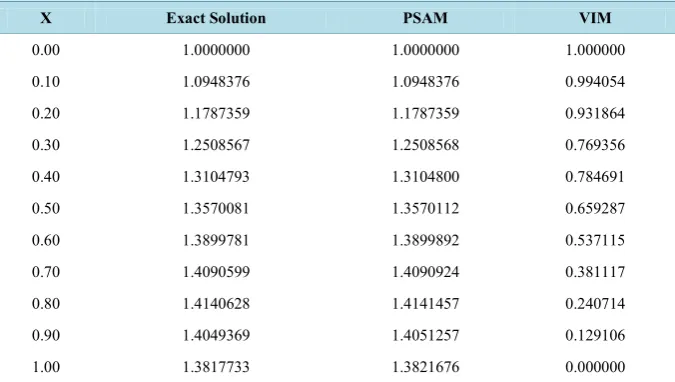
The comparison of the approximate solution of example 1 obtained with the help of PSAM and the approx-imate solution using VIM obtained in [1] is given in Table 1. From the numerical results, it is clear that the PSAM is more efficient and accurate. By increasing the order of approximation more accuracy can be obtained.

Example 2

Consider the following linear tenth-order problem [2]

( )10

_{( )}

_e x 2

_{( )}

_, _.

y x ₌ − y x a x b_{≤ ≤} ₍₃₃₎

with the following boundary conditions

( )

_{( ) ( )}

2k ₀ _{1 ,} _{0,1, 2,3, 4.}

y = k= (34)

( )2k

_{( ) ( )}

₀ _{1 ,} _{0,1, 2,3, 4.}

y = k= (35)

The exact solution is

( )

ex

y x = .

(7)

( )

1

1 2

2 3

2

d _,

d

d _,

d

d _,

d d _e

d x

y y x

y _y

x

y _y

x

y _{y x}

x

−

=

with the boundary conditions at x=ξ0=0

( )

1 2 3 4 5

6 7 8 9 10

0 1, 0 1, 0 1, 0 1, 0 1,

0 , 0 , 0 , 0 , 0 .

y y y y y

y a y b y c y d y e

= = = = =

Since, ξ =0 0, we have Equation (14) as

, 0. ! n n

a n

n λ

= ≥

Hence for n=0 1 9

( )

we have

0 1 2 3 4 5

6 7 8 9

1 1 1

1, 1, , , , ,

2 6 24 120

, , , .

720 5040 40320 362880

a

a a a a a a

b c d e

a a a a

= = = = = =

= = = =

Hence, substituting the above values of a n_n, =0 1 9

( )

in (7), we obtain

( )

₁ 1 2 1 3 1 4 1 5 1 6 1 7 1 8 1 9

2 6 24 120 720 5040 40320 362880

y x = + +x x + x + x + ax + bx + cx + dx + ex (36)

Using boundary condition at x=ξ1=1 on equation (36) we obtain the values of a, b, c, d and e, as

1.000029332

a= , b=0.9997112299, c=1.002812535, d =0.9735681663, and e=1.218281800

Thus, the final approximation solution of the BVP (33) can be written as

( )

2 3 4 5 6

7 8 7 9

1 1 1

1 0.008333577767 0.001388487819

2 6 24

0.0001989707411 0.00002414603587 3.357258047 10

y x x x x x x x

x x E − x

= + + + + + +

+ + +

_{( )}

1

1 2

2 3

3 2

d _,

d

d _,

d

d _,

d

d _2e _,

d x

y y x

y _y

x

y _y

x

y _{y x} _y _x

x

=

= +

with the boundary conditions (at x=ξ0=0)

( )

1 2 3 4 5 6 7

8 9 10 11 12

0 1, 0 , 0 1, 0 , 0 1, 0 , 0 1,

0 , 0 1, 0 , (0) 1 and 0 .

y y a y y b y y c y

y d y y e y y f

= = = = = = =

= = = = =

Since, ξ =0 0, we have Equation (14) as

, 0. ! n n

a n

n λ

= ≥

Hence for n=0 1 11

( )

we obtain the following

0 1 2 3 4 5 6 7

8 9 10 11

1 1 1

1, , , , , , , ,

2 6 24 120 720 5040

1 _, _, 1 _, _.

40320 362880 3628800 39916800

b c d

a a a a a a a a a

e f

a a a a

= = = = = = = =

= = = =

Hence, substituting the above values of a n_n, =0 1 11

( )

in (7), we obtain

( )

2 3 4 5 6 7

8 9 10 11

1 1 1 1 1 1

1

2 6 24 120 720 5040

1 1 1 1

40320 362880 3628800 39916800

y x ax x bx x cx x dx

x ex x fx

= + + + + + + +

+ + + + (40)

Using boundary condition at x=ξ1=1 in Equation (40) we obtain the values of a, b, c, d, e and f, as

0.9999940293

a= − , b= −1.000058885, c= −0.9994190942, d= −1.005725028, e= −0.9434337955 and 1.632120555

f = − .

Thus, substituting the values a, b, c, d, e and f in (40), the final approximation solution of BVP (37) can be written as

( )

2 3 4

5 6 7 8

9 10 8 11

1 1

1 0.9999940293 0.1666764808

2 24

1 1

0.008328492452 0.0001995486167

720 40320

1

0.000002599850627 4.088806104 10 3628800

y x x x x x

x x x x

x x E − x

= − + − +

− + − +

− + −

The comparison of the approximate solution of Example 3 obtained with the help of PSAM and the approx-imate solution using HPM [2] is given in Table 3. From the numerical results, it is clear that the PSAM is more efficient and accurate. By increasing the order of approximation more accuracy can be obtained.

5. Conclusion

(9)

[image:9.595.145.483.101.292.2]

Table 1. Comparison of results of PSAM with Variational Iteration Method (VIM).

X Exact Solution PSAM VIM

0.00 1.0000000 1.0000000 1.000000

0.10 1.0948376 1.0948376 0.994054

0.20 1.1787359 1.1787359 0.931864

0.30 1.2508567 1.2508568 0.769356

0.40 1.3104793 1.3104800 0.784691

0.50 1.3570081 1.3570112 0.659287

0.60 1.3899781 1.3899892 0.537115

0.70 1.4090599 1.4090924 0.381117

0.80 1.4140628 1.4141457 0.240714

0.90 1.4049369 1.4051257 0.129106

1.00 1.3817733 1.3821676 0.000000

Table 2. Comparison of results of PSAM with HPM.

X Exact Solution PSAM HPM

0.0 0.100000000 0.100000000 0.1000000000

0.2 0.122140276 0.122140276 0.1221408246

0.4 0.149182470 0.149182470 0.1491833581

0.6 0.182211880 0.182211878 0.1822127686

0.8 0.222554093 0.222554055 0.2225546413

[image:9.595.144.484.463.574.2]

1.0 0.271828183 0.271827885 0.2718281799

Table 3. Comparison of results of PSAM with HPM.

X Exact Solution PSAM HPM

0.0 10.000000000 10.000000000 10.000000000

0.2 8.187307531 8.187318703 8.187308703

0.4 6.703200460 6.703218540 6.703208540

0.6 5.488116361 5.488134449 5.488114451

0.8 4.493289641 4.493300834 4.493289646

1.0 3.678794412 3.678794408 3.678794453

References

[1] Adeosun, T.A., Fenuga, O.J., Adelana, S.O., John, A.M., Olalekan, O. and Alao, K.B. (2013) Variational Iteration Me- thods Solutions for Certain Thirteenth Order Ordinary Differential Equations. Journal of Applied Mathematics, 4, 1405-1411. http://dx.doi.org/10.4236/am.2013.410190

[2] Othman, M.I.A., Mahdy, A.M.S. and Farouk, R.M. (2010) Numerical Solution of 12th Order Boundary Value Prob-lems by Using Homotopy Perturbation Method. Journal of Mathematics and Computer Science, 1, 14-27.

[3] Watson, L.M. and Scott, M.R. (1987) Solving Spline-Collocation Approximations to Nonlinear Two-Point Boundary Value Problems by a Homotopy Method. Journal of Mathematics and Computation, 24, 333-357.

http://dx.doi.org/10.1016/0096-3003(87)90015-4

(10)

[5] Siddiqi, S.S. and Iftikhar, M. (2013) Numerical Solution of Higher Order Boundary Value Problems. Abstract and Ap-plied Analysis, 2013, Article ID: 427521. http://dx.doi.org/10.1155/2013/427521

[6] Siddiqi, S.S. and Iftikhar, M. (2013) Solution of Seventh Order Boundary Value Problems by Variation of Parameters Method. Research Journal of Applied Sciences, Engineering and Technology, 5, 176-179.

[7] Iftikhar, M., Rehman, H.U. and Younis, M. (2014) Solution of Thirteenth Order Boundary Value Problems by Diffe-rential Transform Method. Asian Journal of Mathematics and Application, 2014, Article ID: ama0114.

[8] Akram, G. and Rehman, H.U. (2013) Numerical Solution of Eighth Order Boundary Value Problems in Reproducing Kernel Space. Numerical Algorithms, 63, 527-540. http://dx.doi.org/10.1007/s11075-012-9608-4

[9] Wu, Y.H., Liu, L., Wiwatanapataphee, B. and Lai, S. (2014) Nonlinear Functional Analysis of Boundary Value Prob-lems: Novel Theory, Methods and Applications. Abstract and Applied Analysis, 2014, Article ID: 754976.

[10] Mamadu, J.E. and Njoseh, I.N. (2016) Numerical Solutions of Volterra Equations Using Galerkin Method with Certain Orthogonal Polynomials. Journal of Applied Mathematics and Physics, 4, 376-382.

http://dx.doi.org/10.4236/jamp.2016.42044