A Method for Setting the Artificial Boundary Conditions of Groundwater Model

A Method for Setting the Artificial Boundary

Conditions of Groundwater Model

Yipeng Zhou1,2, Zhaoli Shen1, Weijun Shi2, Jinhui Liu2, Yajie Liu2 1

School of Water Resources and Environment, China University of Geosciences, Beijing, China 2

Department of Civil and Environmental Engineering, East China Institute of Technology, Nanchang, China Email: [email protected], [email protected]

Received 2013

ABSTRACT

Numerical simulation technology is nowadays an important means for groundwater issues because of its efficiency and economical advantages. But in case of natural hydrogeological boundaries are not within the interest area, it may be a big trouble to set boundary conditions of the model artificially without enough field investigation information. This pa-per introduced a method for solving such problem applying field pumping test and recovery test. The method was ap-plied to build an in-situ leaching of uranium model. Results showed that the model boundary conditions can be set sat-isfactorily, and also the calculated heads matched the observed data well in both two models.

Keywords: Groundwater; Numerical Model; Artificial Boundary Conditions

1. Introduction

Since the 1960s, with the development of computer technology, the method of numerical simulation had been widely used to solve groundwater flow and solute trans-port problems because of its effectiveness, flexibility and relatively economical with spend, and gradually become an important method for groundwater issues [1-7]. However, although lots of models have been built in various applications, few people care about the real ef-fects of those models in practices [8]. One of important factors influencing the reliability of the groundwater model is geology and hydrogeology investigation; and usually making reasonable understandings on boundary conditions is a big challenge [9]. Once the boundary conditions are distorted to the truth, it is bound to lead to significant deviation of the model calibration parameters from actual values, and then serious impact on the reli-ability of the model would not be avoided.

Model boundary conditions are usually set according to field investigations. When the interest area is small that the model boundaries are far away from natural hy-drogeological boundaries, artificial model boundary con-ditions need to be set according to a long-term observa-tion of groundwater at those boundaries. However, in many cases, the required observation data are often un-available; in this dilemma, one alternative way is to ex-pand model extent so that the groundwater can be as-sumed not to be affected by human activities (such as pumping test) taken placed in the interest area; then the

boundary conditions of first type or of second type can be set at model’s boundaries [9]. But this kind of solution also has shortcomings, one of which is that to establish of model hydrogeology configuration beyond the interest area without supplementary geology investigation infor-mation may bring unexpected serious error to the simula-tion results [10,11]. In this paper, in order to build a flow model of groundwater and leaching solution during in- situ leaching of uranium process, a method has been em-ployed to set artificial model boundaries by combining theoretical calculation according groundwater unsteady flow theory and the model iterative calibration using ob-servation data of pumping test and recovery test inde-pendently.

2. Methods

2.1. Basic Principles

2.2. Functions of the Model Boundary Heads

During pumping test in the confined aquifer, draw down lead to the formation of the cone of depression of pres-sure head. The range of cone expands continuously with pumping, and gradually achieves a relative stable state. When the whole model is located within the cone, heads at model boundaries would vary with time; so obviously, model boundary conditions need to be set according to head changes. Therefore, the function of head variation must be got at first.

According to the theory of confined water’s unsteady flow towards to fully penetrating well, the variation of the head drawdown within pumping influence scope can be approximately described by Jacob Formula [12], as in

2 * 2.25 ln 4 Q s T r  Tt 

 (1)

where s is the head drawdown; Q is the pumping rate; T is the coefficient of transmissibility; t is the pumping time; r is the distance to pumping well; μ * is the coeffi-cient of storage.

Thus, the live head can be calculated via Equation (2): 0

( , )_S ( , ) ( , )

H r t H r t s r t (2) where H r t( , )_S is the head at the point with the dis-tance of r to the pumping well and at the time of t;

0 ( , )

H r t is the initial head at the point with the distance of r to the pumping well; s r t( , ) is the head drawdown at the point with the distance of r to the pumping well and at the time of t.

Since in Equation (2) the head is a continuity function of time, it can not to be applied to set model boundary conditions yet; it need to be temporally discretized to n periods, and in each period the head is a constant, thus, the variation of the head drawdown can be described by Equation (3):

1 0 1

2 1 2

1 , , ( , ) ... ,

n n n

s t t t s t t t s r t

s t t t     _{ }      _{ }  (3)

So, the live head anywhere within the cone of depres-sion during pumping test can be given by the piecewise constant function as Equation (4):

0 1 0 1

0 2 1 2

0 1 ( , ) , ( , ) , ( , ) ... ( , ) , S

n n n

H r t s t t t

H r t s t t t

H r t

H r t s t _ t t

     _{  }      _{  }  (4)

Divide the simulation time to n stress periods, and in each period set the model boundary head according to the corresponding constant value of each definition domain

of the function shown in Equation (4).

2.3. Calibrations of the Model Boundary Conditions

After initial boundary conditions being set through the theoretical calculation mentioned above, run the model to calibrate boundary conditions and parameters iteratively using observation data of the pumping test and recovery test independently. The flow chart of the calibration process is shown in Figure 1.

First, build groundwater flow model of the pumping test and set the model initial boundary conditions for iteration according to Equation (4).

Then, run the model built in the former step to cali-brate model parameters and boundary conditions by the observation data of the pumping test. If the standard error of estimate (S.E.E) exceeds 5%, the hydrogeology pa-rameters and boundary conditions would be adjusted slightly and then the calibration repeats. When the S.E.E is below 5%, the calibration process goes to the next step.

Finally, build groundwater model of the recovery test applying the calibration results of the second step as ini-tial state; run it to calibrate model parameters and boundary conditions again using the observation data of the recovery test. The S.E.E of 5% also is applied as calibration error criterion; if results meet the criterion, the calibration process ends and the model parameters and boundary conditions are fixed; otherwise, return to the first step, modify the model parameters and boundary conditions and then the whole process repeats again.

3. Application Example

3.1. Backgrounds and Model Overview

The study was conducted at the piedmont alluvial slope in the southern region of the Turpan-Hami basin. The

interest confined groundwater system has stable imper-vious roof and base; the groundwater flew from south-west to northeast with a hydraulic gradient of 0.02, and was mainly recharged indirectly by the Quaternary phreatic water from the southern mountainous bedrock fissure. The studied issue was about simulation of groundwater and leaching solution flow in the ore-bear- ing aquifer at an in-situ leaching of uranium site. There are five wells (Figure 2); the well CK1 was for extrac-tion, and the rests were for leaching solution injection.

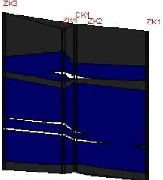
The hydrogeology characteristic of the aquifer within the mining scope is as shown in Figure 3. The average thickness of the aquifer is about 40m; the stable imper-vious roof and base are mainly of mudstone and silty mudstone (in gray); in the aquifer (in blue) there are four discontinuous interlayer, one is of silty mudstone (shown in gray) with the thickness of 1 - 3 meters, and the three others are of calcareous sandstone with the thickness of 0.3 - 0.9 m (in white).

Field pumping test and recovery test were conducted employing well CK1 for pumping, well ZK1 and well ZK3 for observation, the test results are shown in Table 1.

Figure 2. The plan view of well distribution.

Figure 3. Cross section of the aquifer.

Table 1 field tests and the hydraulic parameters of the aq-uifer.

Field test

Test time (min)

Pumping rate (m3_/h)

Coefficient of transmissibility

(m2_/d)

coefficient of storage

Pumping test 2900 7.2

Recovery test 2770 － 0.57 1.95 × 10

-4

Based on those field investigations, the conceptual model of the groundwater flow during the pumping test was built as Equation (5):

0

( ) ( ) ( )

, ( , , ) , 0 ( , , , ) ( , , ) ( , , ) ( , , , ) ( , , , ) ( , , )

xx yy zz

s

S

H H H

K K K

x x y y z z

H

S x y z D t

t

H x y z o H x y z x y z D

W

H x y z t f x y z t x y z S

  _   _   

 

      _

 

   _

 _

  



 _{ }

(5)

where Kxx, Kyy and Kzz are respectively the conductivities

in x, y and z direction in the three-dimension space; H is the confined water head; W is the flux rate per unit vol-ume, which is used to describe the flow rate of wells; Ss is the specific storativity; t is the time; H0(x,y,z) is the initial head at position with the coordinate (x, y, z);

( , , , )_S

H x y z t is the head at the model boundary. The model area denoted D and boundary S.

The initial head of H0(x, y, z) was set according to static water level observed at the beginning of the pump-ing test. Since the modelpump-ing area was small, its edges are far away from the natural hydraulic boundaries known, hence artificial boundaries were necessary. A circle sur-rounding the well CK1 and with radius of 100 meters was set as the boundary of the model.

3.2. Head Functions of the Model Boundary

In case of the coefficient of transmissibility is 5.7 m2/d, the coefficient of storage is 1.95 × 10 – 4 and the pumping rate is 7.2 m3/h, the radius of influence of the pumping test is more than 800 meters; clearly, the heads at the pumping test model boundaries which were 100 meters away from the pumping well must to be varying with time. Calculation according to Jacob formula showed that head drawdown started to take place at the model boundaries after pumping for 3.65 hours. The drawdown function can be derived from Equation (1), as in

0, 0 3.65

2.34 ln 2.95, 3.65 50 t

s

t t

  

  _{  }

 (6)

to approximately replace the curve of the original func-tion s(t), making sure the difference between the two adjacent constants of the function s t( ) was not greater than 0.5 m. The function values are listed in Table 2.

And then, divided the whole simulation time of the pumping test into 15 periods according to the function

( )

s t , in each period initial boundary heads of the model were set as a corresponding constant value, which could be get from the Equation (4) by replacing the values of function s t( ) listed in Table 2 for the drawdown. Then, the iterative calibration process started.

3.3. Results

After correcting the model parameters and boundary conditions repeatedly via the calibration processes of the pumping test model and recovery test model, the model parameters and boundary conditions were fixed on. Re-sults showed that the calculated heads matched the ob-served data satisfactorily in both two models (Figure 5 and Figure 6); the mean absolute error between the cal-culated heads and observed data of pumping test simula-tion was 0.694 m, and recovery test simulasimula-tion 0.655 m; both variances were less than 5%. Furthermore, the coef-ficient of transmissibility was 5.3 m2/d; it was close to the results of field tests (5.7 m2/d).

Figure 4. The curves of function s (t) and functions'(t).

Table 2. The values of function s'(t).

t (h)

) ( ' t

s

(m) t (h)

) ( ' t

s

(m)

t (h)

) ( ' t

s

(m)

0 - 4 0 8 - 10 2.08 22 - 26 4.39

4 - 5 0.5 10 - 12 2.56 26 - 30 4.75

5 - 6 0.91 12 - 14 2.95 30 - 34 5.07

6 - 7 1.32 14 - 18 3.44 34 - 42 5.47

7 - 8 1.66 18 - 22 3.96 42 - 50 5.91

Figure 5. The results of calculated heads matched to ob-served heads of the pumping test model.

Figure 6. The results of calculated heads matched to ob-served heads of the recovery test model.

4. Conclusions

The boundary condition is one of key factors influencing the reliability of groundwater model. In case of artificial boundary conditions are needed, they should be set rea-sonably using as much field investigation data as we can get, otherwise, it is prone to cause great distortion to the truth and make the model worthless. Study results show that the method introduced in this paper can be a feasible choice to set artificial boundary conditions of the groundwater model.

5. Acknowledgements

Thanks for the fund of the Major State Basic Research Development Program of China (973 Program) (No. 2012CB723101).

REFERENCES

Beijing, 1975, pp. 1-8.

[2] H. R. Zhang, “Groundwater Hydraulics Development,” Geology Publishing House, Beijing, 1992, pp. 1-10.

[3] E. M. Labolle, A. A. Ahmed and G. E. Fogg, “Review of the Integrated Groundwater and Surface Water Model (IGSM),” Ground water, Vol. 41, No. 2, 2003, pp. 238-246.doi:10.1111/j.1745-6584.2003.tb02587.x [4] L. H. Wei, L. C. Shu and Z. C. Hao, “The Present

Situa-tion and Development Tendency of Groundwater Flow Numerical Simulation,” Journal of Chongqing University, Vol. 23, 2000, pp. 50-52.

[5] J. H. Ding, D. L. Zhou and S. Z. Ma, “The State-of -Art and Trends of Development of Groundwater Modeling Software Abroad,” Site Investigation Science and

Tech-nology, No. 1, 2002, pp. 37-42.

[6] L. C. Xu, “Introduction to Common Software Products Modeling Groundwater,” Uranium Mining and

Metal-lurgy, Vol. 21, No. 1, 2002, pp. 33-38.

[7] H. Q. Qu, S. Zeng and H. L. Liu, “Research Status and

Development of Numerical Simulation of In-situ Leach-ing of Uranium,” Sci-tech Information Development &

Economy, Vol. 21, No. 9, 2011, pp. 177-180.

[8] Y. Q. Xue, “Present Situation and Prospect of Ground-water Numerical Simulation in China,” Geological

Jour-nal of China Universities, Vol. 16, No.1, 2010, pp. 1-6. [9] W.X. Lu, “Approach on Boundary Condition in

Numeri-cal Simulation of Groundwater Flows,” Journal of

Hy-draulic engineering, No. 3, 2003, pp. 33-36.

[10] Y. Y. Shen and Y. Z. Jiang, “Research on Disposal Method of Artificial Boundary Condition in Numerical Simulation of Groundwater Flow,” Hydrogeology and

Engineering Geology, No. 6, 2008, pp. 12-15.

[11] De lange W. J. and A. Cauchy, “Boundary Condition for the Lumped Interaction Between an Arbitrary Number of Surface Waters and a Regional Aquifer,” Journal of

Hy-drology, 1999, pp. 261-262.

REFERENCES

[image:4.595.61.287.402.565.2] [image:4.595.57.286.607.735.2]Beijing, 1975, pp. 1-8.