House Market in Chinese Cities: Dynamic Modeling, In Sampling Fitting and Out of Sample Forecasting

Munich Personal RePEc Archive

House Market in Chinese Cities:

Dynamic Modeling, In-Sampling Fitting

and Out-of-Sample Forecasting

Leung, Charles Ka Yui and Chow, Kenneth and Yiu,

Matthew and Tam, Dickson

City University of Hong Kong, Hong Kong Institute of Monetary

Research, Hong Kong Monetary Authority

2010

House Market in Chinese Cities: Dynamic Modeling,

In-Sampling Fitting and Out-of-Sample Forecasting

Charles Ka Yui Leung City University of Hong KongΩ

Kenneth K. Chow

Hong Kong Institute for Monetary Research

Matthew S. Yiu

Hong Kong Institute for Monetary Research Hong Kong Monetary Authority

Dickson C. Tam

China International Capital Corporation Limited

December 2010

♣

Acknowledgement: We are very grateful to the comments and suggestions by the referees and seminar participants of AsRES meeting and the HKMA. Leung is grateful to the financial support from the City University of Hong Kong, Chow and Yiu are grateful to the support from HKMA and HKIMR. The views expressed in this paper are solely those of the authors and do not necessarily reflect those of the CICC, HKIMR, HKMA, its Council of Advisors or Board of Directors.

Ω _{Correspondence: Leung, Department of Economics and Finance, City University of Hong Kong,}

Abstract

This paper attempts to contribute in several ways. Theoretically, it proposes simple

models of house price dynamics and construction dynamics, all based on

forward-looking agents’ maximization problems, which may carry independent

interests. Simplified version of the model implications are estimated with the data

from four major cities in China. Both price and construction dynamics exhibit strong

persistence in al cities. Significant heterogeneity across cities is found. Our models

out-perform widely used alternatives in in-sample-fitting for all cities, although

similar success only limited to highly developed cities in out-of-sample forecasting.

Policy implications and future research directions are also discussed.

Keywords: pre-sale, production constraint, collateral constraint, cross-city heterogeneity, fundamental versus policy

1. Introduction

The China property market has experienced an unprecedented growth in the last few

years.1 From 1998 to 2007, the property price index increased by more than 50%.

Moreover, it has been related to the aggregate economy in many important

dimensions, in the manner similar to many developed economies. An obvious

example is the consumer price inflation. According to Peng, Tam and Yiu (2008), the

property price was the second largest contributor to the upsurge in China inflation in

the period from 2002 to 2004. And, as in the United States and many OECD countries,

the property market also contributes significantly to public finance.2 After the

abolition of the administrative housing allocation system in 1998 and the

implementation of the auction policy for land, the revenue from land sales became an

important source of income to both the local and central governments in China.3 The

property market also appears in the discussion of the development and stability of the

banking sector, as in the case of other countries.4 For instance, Deng and Fei (2008)

find that the ratio of mortgage loan balances to total bank loans increased from 0.5%

1

The rapid urbanization and high GDP growth have been pushing forces of this real estate market boom in China recently. The expansion of the mortgage business, which provides sufficient liquidity to the market, might also have played a significant role in boosting the property market. Moreover, the People’s Republic of China implemented a policy in 1998 to encourage the commercial banks to expand the mortgage business and provide financial support to housing consumption after the elimination of the welfare house distribution policy, which is entitled “Management Provisions on Residents Housing Loan” according to Leung and Wang (2007). Over 60% of the real estate investment is financed by bank loans (Liu and Huang, 2004). Peng, Tam and Yiu (2008) also find that the growth of rental price, land price, inflation and GDP are exerting a positive impact on the real estate market.

The focus of this paper, however, is not on the growth of the property market itself, but rather how well a market-based economics model can explain the property market in China.

2

Clearly, it is beyond the scope of this paper to review the literature on this topic. Among others, see Hanushek (2002, 2006), Ross and Yinger (1999) and the references therein.

3

This revenue is even more important for the local government since 40% of the revenue goes to the central government while the local government takes the rest (Chan, 1999). For the case of the United States, see Hanushek and Yilmaz (2007a, b), among others.

4

in 1998 to more than 10% in 2004. The housing wealth also constitutes a large share

and plays a very important role in the household portfolio in China, as many recent

works have recognized in other developed countries.5 For instance, Liu and Huang

(2004) report that home equity took about 47.9% of the Chinese household wealth in

2002 according to an urban survey of National Bureau of Statistics of China. In 2003,

the central government announced the real estate sector as one of the pillar industries

of the Chinese economy, which seems to be an unprecedented official statement both

in the economic history of China and among socialist countries. All these demonstrate

two facts. Apparently the importance of the property market in the Chinese Economy

is growing. In addition, the role of the property market in the aggregate economy in

China has become increasingly similar to the case of other developed countries. Thus, to complement the voluminous empirical literature on the China real estate

market,6 this paper attempts to contribute in several ways.

1. Most of the literature is purely empirical. For those containing theoretical

models, they are either static or at most two periods. In contrast, this paper

provides two infinite-horizon models in which agents are forward-looking and

the first order conditions that we derive naturally tied the choice variables

(such as how much housing to consume) to the market variables (such as the

prices and interest rate).

2. Most of the literature is in reduced form regression. In this paper, we first

derive first-order-conditions (FOC) from agents’ dynamic optimization

problems. We then estimate a linearized version of those first order conditions.

This is in line with the “structural estimation” literature promoted by Hansen

(1982), Hansen and Sinleton (1982), and recently, Piazzesi, Schneider and

Tuzel (2007). (Singleton (2006) provides a textbook treatment on such an

approach.) This approach provides us a “micro-foundation” for the empirical

work and a more explicit linkage between the theory and the empirics.

5

Once again, this literature is too large to be reviewed here. Among others, see Cocco (2004), Yao and Zhang (2005), Piazzesi, Schneider and Tuzel (2007).

6

3. The dynamic models we provide, including the one in the appendix, are

general in nature, and could be modified for other applications. Thus, it may

carry some independent interests.

4. This paper performs out-of-sample-forecasting (OSF) and finds that the simple

models proposed here match the data reasonably well. To our knowledge,

most empirical works on China do not perform OSF. (The importance of OSF

have been discussed by Meese and Rogoff, 1983; Cheung, Chinn and Pascual,

2005, among others).

5. Perhaps even more importantly, this research strategy will test empirically

whether real estate economics models developed in the tradition of the main

stream economics are capable to account for the dynamics of the China

property market. Given the fact that the Chinese real estate market is

constantly exposed to frequent and discretionary government intervention,7 and the well known micro-level differences,8 it is not clear why models that are developed to explain the advanced economies will also be applicable in the

Chinese economy, unless the market in China has indeed reached a certain

level of maturity. To put it in another way, the economic reforms in China are

now “significant enough to be detected” in the real estate market.

The house price and construction dynamics are chosen to be the focus of

this study for obvious reasons. First, the China housing price and construction data

series in China are more complete than other related series. Second, they are also

more “visible” for the general public and the media, and therefore often are chosen as

policy targets of the government. Limited by the data availability, we focus on the

data series from four major cities, we can afford to estimate them separately and be

able to present the results clearly. In particular, we would compare whether during a

fixed sampling period, the same set of variables would have similar impact on the

price and construction dynamics across different cities. In addition, we will conduct

out-of-sample forecasting and compare the performance of our models with some

7

See Leung and Wang (2007), Deng and Fei (2008), and the references therein, for more details.

8

widely used alternatives. To our knowledge, thus far there has been no attempt to

conduct empirical test which are directly derived from maximization modes, and to

conduct both in-sample-fitting and out-of-sample forecasting for China housing

market at the city level. This paper takes an initial step towards this direction.

The reasons to focus only on the quarterly data from four major Chinese

cities, namely, Beijing, Tianjin, Shanghai and Chongqing, from 1998 to 2008 are

clear. Their data series are relatively longer (which will enhance the study of market

dynamics) and they are also relatively more developed in China. Their housing

markets are expected to be more market-driven so that the model should be more

applicable to these cities. Our approach reflects our assumption that housing markets

in cities at different stages of economic development and different industrial

specialization may behave differently. To complement the previous literature, which

are either based on cross-sectional regressions, or the panel data approach with

city-fixed effects, this paper would rather study these cities separately, and thus

allowing the quantitative relationships among variables are indeed very different

across cities. In fact, our results seem to justify our “priors” and we will explain the

results in details in the following section.

The organization of this paper is as follows. Section 2 describes the

methodology. The details of the regression equations we use, different estimation

approaches and the estimation issues will be discussed in this section. Section 3

presents the empirical results and discussions. The final section will discuss the policy

implications and conclusions.

In this paper, we intend to build two simple dynamic models, one for the housing

price and one for the construction. And based on the theoretical results from those

models, we will propose two simple empirical models, which will in turn be estimated

with the China data. We will assess the performance of those empirical models based

on both in-sample fitting and out-of-sample forecasting. In this section, we will first

present the theoretical model of house price, followed by the empirical counterpart.

We then switch to a simple model of construction, which will also be followed by its

empirical counterpart.

2.1 A simple Model of House Price

This section proposes a simple model of city level house price, which would

provide some guidance for our empirical investigation. Following the

consumption-based house price model of Kan et al (2004), Leung (2003, 2007), we

assume that there is a forward-looking, representative consumer in a city, which

maximize the lifetime utility

(

)

0

max t _t, _t

t

U C H

β ∞ =

∑

each period, with β∈

( )

Greenwood and Hercowitz (1991), we assume that the utility function is separable in

the non-durable consumption C_t and the housing stock H_t,

  U C H

(

)

where ω>0is the parameter governs the relative importance of non-durable

consumption C_t and the housing stock H_t in the utility function. To ensure

“time-consistency,” we adopt the dynamic programming approach in solving the

model. The Bellman equation for the dynamic optimization can be written as

  V H W P P

(

)

(

)

(

)

  W_t+P H_{t t}s ≥C_t+γP H_{t t}s₊₁+ −

(

)

where W_tis the wage, P_t is the per unit house price, s t

H is the stock of housing

purchased in the previous period and owned in the current period, γis the

down-payment ratio, R_t is the interest factor imposed on the mortgage carried from

period (t-1) to period t, h t

R is the rent for rental housing, r t

H is the amount of rental

housing for the current period. For simplicity, we simply assume that the consumer

treats the owner-occupied housing s t

H and rental housing r t

H as perfect substitute.

  s r

t t t

H =H +H  

This formulation of budget constraint follows both Kan et al (2004) and Chen, Chen

and Chou (2010). It simply formulates the idea that the total revenue (the left hand

side of (1)), which is the sum of the wage and the re-sale value of the house, should

exceed the total expenditure (the right hand side of (1)), which is the sum of the total

value of consumption, the down-payment for the house purchase in the current period,

and the mortgage debt carried from the last period.

Following the method in Kan et al (2004), the first order conditions are easy to

derive,

  λ_t =1 /C_t, 

  1

(

)

h s r

t t t

t

R H H

λ ω

+ = , 

{

( )

(

)

}

t Pt Ht t Pt R Pt t

λ γ =β ω ₊ − +λ₊ ⎡_{⎣ +} − −γ ₊ ⎤_⎦ . 

(

)

1 1 1

1 1

1

t t t

t s

t t t t

P C C

R P C P H

γ _{ω γ}

β + + + + + ⎛ ⎞ ⎛ ⎞ ⎛ ⎞ =_{⎜ ⎟⎜ ⎟}− _{⎜ ⎟}+ − ⎝ ⎠⎝ ⎠ ⎝ ⎠ ,

(

)

h s r

t t t

t

R H H C

ω

+ = .

Or, the two expressions can be combined as

(

)

1 1 1 1 1

1 1

1

h s r

t t t t t

t

h s r s

t t t t t t

P R H H C

R P R H H P H

γ _{ω γ}

β + + + + + + + ⎛ ⎞⎛ ⎞ ⎛ ⎞ ⎛ ⎞ + =_{⎜ ⎟⎜ ⎟⎜ ⎟}− _{⎜ ⎟}+ − +

⎝ ⎠⎝ ⎠⎝ ⎠ ⎝ ⎠ . (1’)

Notice that most variables in (1’) are available and hence in principle, we can directly

estimate (1’) with GMM or other nonlinear econometric technique. However, with

only 40 quarterly data points, it is difficult, if not impossible, to do so. Following the

log-linear approximation method of King, Plosser and Rebelo (2002), the equation

above can be roughly approximated as

฀

1

1 0 1 1 2 1 3 4 1

1

h t

t t t s t

t t

C

GP a a GR a GH a a R P H + + + + + + ⎛ ⎞ = + + − _{⎜ ⎟}+

⎝ ⎠ . (2)

Thus, this simple model suggests that the growth rate of house price GP_t+1 is related to the growth rate of the house rent GR_th₊₁, the growth rate of the housing stock GH_t+1, a change of the ratio between the expenditure on non-durable

consumption versus the value of the housing wealth

฀ 1 1 t s t t C P H + + ⎛ ⎞ ⎜ ⎟

⎝ ⎠ , and the mortgage

interest rate R_t+1. Clearly some of the variables such as GP_t+1 and GR_th₊₁, are much more accessible to the authors than the others. In the next section, we will discuss in

more details how the empirical work is implemented.

This section attempts to study the housing market dynamics of some major cities in

China. Our estimation is “linear in form” and “structural” by nature. Inspired by the

simple theoretical analysis of the previous section, we envision that the housing price

follows the following process,

1 2 4 1

[ ] (1 )

t t t t t

GP=ϕ γ GR +γ GWAGE +γ DU + −ϕ GP₋ (3) where GP is the growth rate of the overall property price index, GR is the annual growth rate of the real rental, GWAGE is the growth rate of household real disposal income, DU is the annual difference of the real lending rate for housing loans as a measure of user cost of homeownership. Roughly speaking, equation (3) is broadly

consistent with growth models with endogenous real estate price (among others, see

Tse and Leung, 2002; Leung, 2003).

The intuition behind this equation is very simple. First, the theoretical result in

the previous section suggests that the growth rate of property price is (intuitively)

related to the growth of the housing rental rate. There are additional reasons why we

would focus on the growth rate of the house price instead of the levels. During our

sampling period, the house price of China has a clear upward trend. Estimating these

potentially non-stationary data series directly may lead to spurious regressions. A

suitable de-trending9 of the level data is therefore appropriate. Moreover, the level

data of the China property price is not available in quarterly frequency. Only the growth rate of the property price at city level is accessible. Thus, focusing on the growth rate of property price is well-justified in all kinds of consideration. This also

helps us to differentiate from some of the earlier efforts which tend to focus on the

cross-sectional difference of the house prices across cities.

9

The other terms in equation (2) are difficult to find accurate quarterly measures

for all cities. Thus, we need to use proxies. First, on a quarterly basis, the total stock

of housing may not change as much as the other variables and we might therefore

switch the attention to the other variables, such as the change of the ratio between the

expenditure on non-durable consumption versus the value of the housing wealth

฀

1

1

t s t t

C P H

+ +

⎛ ⎞ ⎜ ⎟

⎝ ⎠. In case of separable utility function, as we assume here, this term is

likely to be stationary over time. However, the utility function of a representative

agent may not be separable in non-durable consumption and housing in practice. In

fact, some empirical works suggest that the utility function is indeed non-separable.10

In the appendix, we solve for the non-separable case and find that it is even more

difficult to find an appropriate proxy in practice. On the other hand, as shown by the

work of Atkeson and Ogaki (1996), Ogaki and Atkeson (1997), the change in the

relative importance of non-durable consumption (such as food) versus housing is

related to the income. Since wage is a non-stationary variable during the sampling

period, we use the growth rate of wage instead.

Another term that appears in equation (2) is the interest rate. As mentioned by

Liu and Huang (2004), over 60% of the real estate investments are financed by bank

loans in China. Thus, the interest rate can be an important factor. Since the interest

rate is non-stationary, we use the annual difference of the real lending rate for housing

loans (DU) will serve as a measure of user cost of homeownership in the regression. The last term reflects that the growth rate of housing price may have some

persistence (and thus GP_t may depend on GP_t−1 ). This can be due to the

informational friction. In contrast to the United States, the information flow is slower

10

and the market transparency is lower.11 It may also be due to behavioral reason such

as momentum, or because of the persistence of technological shocks, or because of

habit formation in the preference.12 Moreover, all of the estimations will be based on

quarterly data. Thus, serial correlation of prices that may not appear in some previous literature (which employ only annual data) may nevertheless be found in quarterly

data.13

Clearly, some other variables may also be important, such as the housing stock

data, the construction data, the evolution of the demography of each city, the

age-dependent home ownership rate, etc. Unfortunately, those variables are not

available for the whole sampling period. By the same token, we are unable to identify

quarterly price data for each type of real estate in each city. Only the overall property

price index can be obtained. Fortunately, in these major cities, the residential property

constitutes more than 60% weight in the overall price index. Moreover, as these cities

are rapidly growing and resources are being intensively competed. As a result, the

prices of different types of property tend to move together. Equation (3) thus

represents a compromise of the “ideal model” we would like to estimate and the data

available for estimation. As it will become clear, despite all these limitations, our

simple model achieves moderate success, as it will be clear in later sections.

The expected signs are the other coefficients are straightforward. With regard to

the rental growth (GR), a positive coefficient is expected because housing can also be regarded as an investment asset. If the rental growth increases, the return on holding

real estate assets becomes higher, which will attract more capital to go into the real

11

For instance, during most of our sampling period, second hand market transaction data are not available from the government, but only through real estate agents, who have strong incentive to selectively report or even mis-report.

12

Among others, see Leung (2007), Leung and Chen (2006) for a discussion and explicit modeling of the equilibrium dynamics of real estate price.

13

estate market and lead to higher housing prices. Similarly, the household disposal

income growth (GWAGE) is expected to have a positive effect on price as faster household income growth will normally generate a greater demand for housing.

A higher growth rate of the interest factor, however, can have different impacts.

On the one hand, if the interest factor grows fast, it will increase the opportunity of

house purchase, and would suppress the growth rate of the house price. On the other

hand, the interest factor is indeed an endogenous variable. The increase in the interest

factor may simply reflect a strong demand in housing (and other assets) and the

central bank in China needs to “intervene” by increasing the opportunity cost of house

ownership. Thus, the net effect of the interest rate change on the house price growth

can go either way, leading to ambiguous prediction on the coefficient in the linear

regression.

2.3 A Simple Model of Construction

The theoretical literature on construction and real estate development is

voluminous and it is clearly beyond the scope of this paper to review it here. Wang

and Zhou (2006), among others, provide an excellent review of the literature. More

recently, the literature also embeds the pre-sale behavior of the developers into the

model, such as Lai, Wang and Zhou (2002), Chan, Fang and Yang (2008), Liu,

Edelstein and Wu (2009), among others. While the simple theoretical model builds on

their insights, it has a very different focus, which is to relate the construction activities

(developer side) to the land price and house price in a dynamic setting. To maintain

the tractability of the model, some simplifying assumptions are made. They can be

justified by the work mentioned above. To explicitly model those choices, however,

Following the work of Kan et al (2004), this section considers a

representative developers who takes the prices as given and maximizes an infinite

flow of profit,

∑

∞ =0

t t tπ

β , where π_t is the profit at time t, which can be expressed in

the following way,

(

)

(

)

h h c l l

t P Ht t P Ht t It P Lt t P L Rt t t

π =α + −α ₊ − −ξ − −ξ _{− −} (4)

The idea behind this expression is simple. We assume that the developer sells a

fraction α, 0<α <1, of the housing units he produced at period t at the market

price h

t

P , i.e. H_t, and pre-sell a fraction (1−α) of the housing units he will

complete at period (t+1), i.e. H_t+1, also at the market price h t

P . Thus, we ignore the

potential “pre-sale discounting” or pricing-in issues, for simplicity. These are the

revenue of the developer. He has three sources of expenditure. On top of the

investment expenditureI_tc, the developer needs to pay for the land, which is necessary

for the construction.14 We assume that the developer receives some kind of short term

loan (“bridging loan”) so that he only needs to pay for a fraction ξ, 10<ξ < , of the

value of land purchased at time t, l _t

t L

P , where L_t is the amount of land the

developer purchases at the market price of land at time t, P_tl. In addition, the

developer needs to pay for the residual amount of the value of land purchased in the

previous period (interest included). Since the developer has already paid for the

fraction ξ of it in the previous period, he only needs to pay the remaining fraction

) 1

( −ξ of it. This is the last term

(

)

14

Notice that we have used “C” to represent non-durable consumption in the previous section, and

The developer faces two constraints. The production constraint dictates the

amount of housing that can be produced given the investment and inputs,

( )

( )

1 1

η η

−

+

≤

c t

t

I

L

H

where 0<η₁,η₂ <1 are parameters governing the marginal product of each input in

the production function. Notice also that land needs to be purchased in period (t-1) while investment is made in period t for the housing to be delivered in period (t+1). This differential in timing captures the observation that some preparation works need

to be done first (including the management of underground water, etc.) before real

construction works are possible.

The second constraint concerns the collateral constraint of the developer.

Previous theoretical work such as Hart and Moore (1994), Chen (2001), and empirical

work such as Chen and Wang (2007, 2008), Wang and Chang (2008), among others,

all suggest that the collateral constraint is important for firms. Empirical finance

researches also suggest that the capital structure may be important in the investment

decisions of firms.15 In the current context, we assume that the value of debt due to

land purchase does not exceed the value of houses that will be completed in the next

period and have not been pre-sold. Formally, it means that

  αP H_t+h_{1 t+1}≥ −

(

)

As in Kan et al (2004), we adopt the dynamic programming approach to

ensure “time consistency” of this maximization problem. The Bellman equation can

be written as

  Ψ

(

)

(

)

15

subject to the constraints (5) and (6), where π_t is given by (4). The first order

conditions are easy to derive with the Kuhn-Tucker Theorem,16

( )

( )

1 1 1

1 c c

t It Lt

η η

λ η − −

=    

(

)

2 1

(.) 1

l c l t

t t t t

t

P P R

L

ξ ξ λ β +

+

⎛∂Ψ ⎞ + − _{= ⎜ ⎟}

∂ ⎝ ⎠ 

( )

(

)

1, 2, 1

1

.

1

c c h h

t

t t t t

t

P P

H

β + λ λ α α

+ +

∂Ψ

= − − −

∂  

where λ₁c_t, λ₂c_t are the Lagrangian multipliers of (5) and (6) respectively, Ψ

( )

(

)

( )

(

)

( )

( )

1 1, 1 2 1

.

1 l c c

t

t t t t t

t

P R I L L

η η

ξ λ η −

+

+ + +

∂Ψ

= − − +

∂ , 

( )

1 1 . _h t t t P H α + + + ∂Ψ = ∂ . 

At the equilibrium, the production constraint, i.e. equation (5), must be binding,

otherwise the profit is not maximized. The collateral constraint, i.e. equation (6),

may not be binding. Therefore we need to study the two cases separately.

Case (a): Collateral constraint is not binding.

In other words, αP H_t+h_{1 t+1}> −

(

)

t

λ = . The dynamical system

can then be reduced to

16

  c ₁c _{1 1}

t t t

I =λ ηH₊ , 

  ξP_tl+ −

(

)

(

)

(

)

(

)

t t t

P P

α α β ₊ λ

− + = .  

They imply that

(

)

(

)

(

)

(

)

2 1 1

1 1

1 2 2

1 1 1 1 1 1 c l t

t t t

c l

t t t t

h h

t t t

h h

t t t

R I P L

I P L R

P P H P P H

ξ ξ β ξ ξ β

α αβ α αβ + + + + + + + + + + + ⎛ + − ⎞ ⎛ ⎞⎛ ⎞ =⎜ ⎟⎜ _⎟⎜⎜ _{+ −} ⎟_⎟ ⎝ ⎠⎝ ⎠⎝ ⎠ ⎛ − + ⎞⎛ ⎞ = ⎜_{⎜ − +} ⎟⎜_⎟ ⎟ ⎝ ⎠ ⎝ ⎠  

       (7) 

which suggests that the growth rate of construction investment will depend on the

growth rate of land price, l₁/ l

t t

P₊ P , the growth rate of land purchase, L_t+1/L_t, and some adjusted ratio of the interest factor,

(

(

)

)

(

(

)

)

in different periods,

(

(

)

(

)

)

(

(

)

(

)

)

t t t t

P P P P

α + α β + α α β +

− + − + . There is,

however, another case that we should also consider.

Case (b): Collateral constraint is binding.

In other words, h_{1 1}

(

)

t t t t t

P H P L R

α _{+ +} = −ξ ₊ and ₂c 0

t

λ > . The dynamical system

will then become

  c ₁c _{1 1}

t t t

I =λ ηH₊ , 

  _2,

1 1 1 1

1 c 1 h

c t t

t h h

t t t

I P

P H P

α

λ β

αη + + α +

⎛ ⎞

(

)

(

)

1 2,

1

1

c

l c t

t t t

t

I

P R

L

η β

ξ ξ λ β

η + +

⎛ ⎞ ⎡ + − + ⎤_{= ⎜ ⎟} ⎣ _{⎦ ⎝ ⎠} . 

The last two expressions together imply that   

(

)

(

)

1 1

2

1 1 1 1

1 1 1 1 1 1 1 1 1 1 1 c l

t t t t

c h

t t t

l h

t t t

t

c h

t t

l h

t t t

t

c h

t t

I P L R I P H

P L P

R

I P

P L P

R

I P

η β ξ

η αη α ξ ξ α α ξ ξ η α + + + + + + + + ⎛ ⎞ ⎛ ⎞ ⎛ ⎞ ₌ ⎛ − ⎞ ⎜ ⎟ ⎜ ⎟ ⎜ ⎟ ⎜ ⎟ ⎝ ⎠⎝ ⎠ ⎝ ⎠⎝ ⎠ ⎡ ⎤ ⎛ ⎞ ⎛ − ⎞ ⎛ ⎞ +_{⎜ ⎟⎢} + − _{⎜ ⎟ ⎜ ⎟⎥} ⎝ ⎠ ⎝ ⎠⎣ ⎝ ⎠⎦ ⎡ ⎤ ⎛ ⎞ ⎛ ⎞ ⎛ ⎞ ⎛ − ⎞ =_{⎜ ⎟}+_{⎜ ⎟⎢} + − _{⎜ ⎟ ⎜ ⎟⎥} ⎝ ⎠ ⎝ ⎠ ⎝ ⎠⎣ ⎝ ⎠⎦ . 

       (8) 

The last equality is due to the fact that h_{1 1}

(

)

t t t t t

P H P L R

α + + = −ξ + . This expression (8)

suggests that the growth rate of construction investment will depend (in a nonlinear

manner) on the growth rate of the house price, P_th₊₁/P_th, the current level of residential investment, the value of land holding P L_tl _t, the interest factor, etc.

2.4 An Empirical Construction Equation

The previous theoretical analysis suggests that the growth rate of the

construction could depend on several factors and whether the real estate developers

are being constrained or not. In a complete market, there is a one-to-one

corresponding between the “price side” and the “quantity side” by the duality

theory.17 In that case, it suffices to study the price dynamics and we can safely ignore

the construction dynamics. Unfortunately, markets are far from being complete in

practice, especially for the China real estate market. Therefore, it is necessary to

17

estimate another equation on the “quantity side” separately. Since our sampling period

is rather short (with less than 40 observations), we restrict our attention to the case of

a linear model.18 Inspired by the theoretical analysis in the above section, we consider

the following equation for estimation.

1 2 3 4 5 1

t t t t t

GC = +δ δ GP+δ DTREAL +δ GLPI +δ GC₋ , (9) where GC is the growth rate of residential commodity building construction started,

GP is the growth rate of the real housing price, DTREAL is the annual difference of the real lending rate. GLPI is the growth rate of the real land price. Clearly, the

corresponding coefficient δ₅ measures the persistence of the growth of new

construction.

The rationale of this equation is straightforward. The theoretical analysis in

the previous section shows that the growth rate of the construction started GC_t

could depend on the growth rate of the house price, the change in the interest factor,

the growth rate of the land price. Therefore, we include those variables in the equation

(9). Obviously, a higher growth rate of the house price will encourage more

construction work to start. A higher growth rate of the interest factor, however, can

have different impacts. On the one hand, if the interest factor grows fast, it will

discourage developers from building new houses. On the other hand, the interest

factor is somewhat endogenous. The central bank in China, just like central banks in

other countries, tends to increase the interest rate when the economy is “hot.” In other

words, there is likely to be a high demand for housing and the central bank attempts to

“stabilize” the market by increasing the interest rate. In other words, an increase in the

interest rate simply represents an underlying strong demand for housing. Thus, the net

18

effect of the interest rate change on the construction growth can go either way,

leading to ambiguous prediction on the coefficient in the linear regression.

The same intuition applies to the growth rate of the land price. Other things

being equal, an increase in the growth rate of land price will increase the construction

cost and hence discourage the construction work to increase. However, other things

are typically not equal. The land price increases because it reflects a strong economic

growth being foreseen or a significant demand increase being perceived. Thus, the

growth rate of construction started can also be positively associated with the growth

rate of the land price.

There are reasons to suspect that housing construction may indeed be

serially correlated. First, housing construction takes time and therefore a single

project may take several periods to be finished, creating a serial correlation in the data.

It is especially true in this quarterly frequency dataset. Also, if the productivity shock

is persistent over time, developers would increase their construction in consecutive

periods, as in Leung (2007).

Notice that the growth rate of price is included in the construction equation

(9), but construction does not enter the pricing equation (3). The reason is very simple.

Price can change instantly while construction may take time to adjust, perhaps due to

some ongoing projects. Thus, even though both house price and new construction are

both endogenous variables from a dynamic equilibrium point of view, the house price can adjust much faster and would capture information about future changes. In this sense, price is a “more forward-looking” variable than the construction level.

Therefore, it makes sense to include price in the construction equation (9) in order to

capture information that may not be available for the econometrican yet are known to

level in the price equation (3) as it may not capture much extra information about the

future.

Again, there are other variables such as the land holding, the amount of

housing stock on the market, etc. that could be included in the construction equation

(9). Unfortunately, data of those variables are not available for the regression.

3. Data and Estimation Results

Our empirical procedures contain two parts. The first part is to study the

housing price and housing construction dynamics in the four major cities in China,

based on equations (3), (9). For the house price equation (3), we estimate the model

with data from 2000Q3 to 2007Q4, the most accessible to the authors for all four

cities (Beijing, Tianjin, Shanghai and Chongqing). For the construction equation (9),

we estimate the model with data from 1998Q2 to 2007Q4. All data used in this paper

are from the CEIC Data Ltd, a data provider whose data are from official sources.

Table 1 and 2 provide some summary statistics. Constrained by the data, we simply

apply OLS on each city separately.19 As we have explained those linear regressions

can be regarded as the linearization of the first order conditions resulted from the two

dynamic models derived from above. Thus, the coefficients estimated from the

regression carries “structural interpretations.” We run the regressions separately for

each city because cities could differ in terms of culture, economic development, legal,

and other infrastructures, which would affect the estimated coefficients. This is our

in-sample-fitting part. The second part is out-of-sample forecasting. We use our

model to forecast the house prices and construction dynamics in 2008 in those four

major cities in China.

19

(Table 1 and 2 about here)

In the literature, there are discussions on whether in-sample-fitting (ISF) or

out-of-sample-forecasting (OSF) should be used as the criteria to measure the

performance of an econometric model (among others, see Meese and Rogoff, 1983;

Inoue and Kilian, 2004; Cheung, Chinn and Pascual, 2005). In this paper, we will

consider both ISF and OSF. And to more accurately assess the performance of our

model, we provide two widely used alternatives for comparison in both ISF and OSF.

We follow the literature to use both RMSE (Root Mean Squared Error) and

MAE (Mean Absolute Error) as the metric for the models’ ability to match with the

data. We will first present the results regarding the house price equation, followed by

those related to the construction equation.

Table 3 presents the regression results regarding the house price equation in

individual cities. All models are adjusted for heteroskedasticity and autocorrelation

by the Newey-West HAC Standard Errors and Covariance.Overall, the model works

well in these four cities. In terms of the more conventional measure, the model applies

pretty well in Beijing, achieving a R2of 0.90. The case for Tianjin and Shanghai are also reasonable good, with a R2of 0.80 or above. The case of Chongqing is a little below the norm, with a R2slightly below 0.60. It may be due to its relatively less developed economy, or due to a very different sectoral focus, and hence our model

may not match that well. The diversity of the model performance also seems to justify

our city-by-city approach.

(Table 3 about here)

For individual variable, the real growth rate of household income has a

positive (and statistically significant) effect on the growth rate on house price change,

as expected. The effect of rental growth is however insignificant. The effect of the

the previous period growth rate of property price is always positively and statistically

significant effect on the house price growth. Such persistence in house price is

consistent with the equilibrium model where technological shocks are persistent and

agents rationally respond to shocks (such as Leung, 2007).

We now turn to the in-sample-fitting. We compare our model with the two

widely used alternatives, namely the 1st degree auto-regressive model (AR(1)) and the

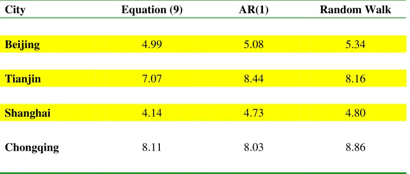
random walk. In terms of RMSE, our model out-performs the alternatives in all four

cities, as shown in table 4a. In terms of MAE, our model still out-performs the

alternatives in all except Chongqing, as shown in table 4b. Putting all these together,

despite the simplicity, our model has apparently captured some important

characteristics of the house price dynamics in these four cities during the sampling

period (2000Q3 – 2007Q4).

(Table 4 about here)

In terms of the out-of-sample forecasting, our model does not do as well. In

terms of RMSE, our model only out-performs the alternatives in Beijing, as shown in

table 4c. In terms of MAE, our model out-performs the alternatives in both Beijing

and Chongqing, as shown in table 4d. One possible explanation is that during the

period of OSF (i.e. the period 2008Q1 -2008Q4), some changes occur in the market of

Tianjin and Shanghai which are not captured by our model. We can only leave this to

future research for more in-depth investigation.

We now turn to the construction equation (9). Table 5 reports the regression

results. Overall, the results are even better than the counterpart of the house price

consistent with the previous literature that dynamic models typically match the

quantity dynamics better than the price dynamics.20

(Table 5 about here)

As we compare the effect of individual variable on the construction growth

rate, we again notice the very significant diversity across cities, even though we are

using the same econometric model. For instance, the growth rate of the property price

has a positive and statistically significant impact on the construction growth in Tianjin.

And the point estimate is 0.99. Thus, the effect from house price to construction is, in

a sense, one-to-one! The counterparts in the other cities, however, are all statistically

insignificant. In the case of the difference of lending rate, the coefficients are negative

and statistically significant in Beijing and Shanghai, which are arguably more

developed. The counterpart of Tianjin is positive and statistically significant. In Chongqing, the coefficient is also large in magnitude and is statistically significant at

10% level. This contrasting result between the relatively more developed cities and

the relatively less developed is also observed in the case of the land price. While they

are all statistically significant at 10% level, the coefficients of the growth rate of land

price are positive in both Tianjin and Chongqing yet negative in Shanghai. Thus, the

level of “market-ization” may affect how the housing started (or other real estate

market variables as well) respond to the changes of the market conditions. And had

we adopted the panel data approach which only uses a city-level fixed effect, we may

not be able to capture such city-level heterogeneity.

Persistence, measured by the coefficient of the lagged construction growth

rate on the current construction growth rate is always positive and statistically

significant. Interestingly, the coefficients for both Beijing and Shanghai are above

0.90, while the counterparts for both Tianjin and Chongqing are between 0.70 and

20

0.80. Thus, even if the effect of a variable is positive in all cities, the magnitude of

that effect can be different across cities.

In terms of the in-sample-fitting (ISF), our model again out-performs the

alternatives in all cities according to RMSE, and in all cities except Chongqing

according to MAE, as shown in table 6a and 6b. Just as the case of house price

dynamics, our construction model seems to capture some important dynamics during

the sampling period (1998Q2 -2007Q4).

(Table 6 about here)

Unfortunately, our out-of-sample forecasting (OSF) is not as successful as

the ISF. In terms of RMSE, our model only out-performs the alternatives in Shanghai,

as shown in table 6c. In terms of MAE, our model out-performs the alternatives in

both Beijing and Shanghai, but not in Tianjin or Chongqing, as shown in table 6d. The

results here are consistent with the previous conjecture that during the period of OSF

(i.e. the period 2008Q1 -2008Q4), some changes occur which are not captured by our

model. We again leave this to future research.

4. Concluding Remarks

Many have been written on the China housing market. This paper

complements the existing literature by providing two simple dynamic models, in

which households and developers are forward looking and respond to prices optimally.

In particular, the household are bounded by the budget constraint and the developer

pre-sells her housing units and is required to meet both the production constraint as

well as the collateral constraint. These models deliver two nonlinear equations

endogenously, one for price dynamics and one for construction dynamics. These

equations relate the house price and construction to other variables, such as the land

applied to different economies, we consider there may be an independent interest for

these two models. In fact, an on-going research project is to further extend and

develop them.

In the context of the major Chinese cities, with less than 40 observations in

each series, we are unable to conduct structural estimation. Instead, we confront the

linearized versions of them to the time series from four major cities in China (Beijing,

Tianjin, Shanghai and Chongqing). We conduct the regression separately and hence

allow the coefficients of the same variable taking different values across cities.

Several empirical results are obtained. Overall, our simple regression

models perform reasonably well. Heterogeneity across cities, on the other hand, is

very dramatic. For instance, in the case of house price equation, while Beijing

achieves a R2 of 0.91, Chongqing achieves 0.59. and while the growth rate of the real household income is positive and statistically significant for both Beijing and

Tianjin, it is marginally significant for Shanghai (10% level) and not significant at all

for Chongqing. Interest factor is important only for Tianjin but not other cities. In the

case of construction equation, growth rate of the property price is positive and

statistically significant for Tianjin, but not significant at all for other cities. The

interest factor will positively and significantly affect the growth rate of construction in

Tianjin and Chongqing, but negatively and significantly in Beijing and Shanghai. The

growth of land price will negatively affect the construction growth in Shanghai, but

positively in Tianjin and Chongqing. These results may suggest that cities in China

are indeed very different, especially in terms of the stage of economic development

and therefore their response to economic environment changes and policy changes

may be very different as well. It also cautious us in the application the Panel data

approach on Chinese city research which only differentiate cities by a city-level fixed

“decompose” the cross-city heterogeneity to differences in institutional factors,

differences in the economic development or sectoral specialization, among other

factors.

While measures such as R2 may give a sense of the “absolute

performance” of the model, we would also like to obtain some measures of “relative

performance” of the model. More specifically, we compare both the in-sample-fitting

(ISF) and out-of-sample forecast (OSF) of the model with two widely used

alternatives, namely, the AR(1) and the random walk. We use both RMSE and AME

to establish the robustness. Interestingly, both of our price dynamics equation and our

construction dynamics equation out-perform the alternatives in ISF in most cases. In

other words, despite their simplicity, both of our price dynamics and construction

dynamics capture some important feature of the data during the sampling period 1998

to 2007. For OSF, however, our price dynamics model consistently out-performs the

alternatives only in Beijing. Similarly, our construction dynamics model consistently

out-performs the alternatives on OSF only in Shanghai. One possibility is that there

are changes occur during the year 2008 that our model fails to capture. We will

continue to investigate this issue in the future research.

The third major empirical finding is that in both price dynamics and

construction dynamics models, the lagged variable are always positive and statistical

significant, although the magnitude varies slightly across cities. One interpretation

from the literature that this is due to the sluggish adjustment of housing stock, which

has been repeatedly documented (among others, see Hanushek and Quigley, 1979;

Leung, 2007). Needless to say, it can also be due to information diffusion (as

information flow in China is not as efficient as in some Western countries), or policy

persistence (as government policy still plays an important role in the housing market).

the causes of persistence in price and construction dynamics, and to identify the role

of policy in the dynamic propagation mechanism.

This paper also carries important policy implications. For instance, if the

housing market is believed to be “overheating,” our results suggest that increasing the

interest rate for mortgage loans may not have a significant direct effect on bringing down the house price growth in the short run. This is because the housing market of

the four cities in the sample period may have been subject to strong speculation or

constrained by credit rationing under macro control policy undertaken by the

government. In principle, the interest rate may have an indirect effect or some general equilibrium effect through its impact on the aggregate output or the stock market. To

address this concern, we will need a more elaborate econometric model for the joint

estimation of the real estate sector and the aggregate economy, which in turn demands

longer time series and more aggregate data.

For another policy application, this paper also shows that the interest rate

and the land price change can have very different impacts on the construction across

cities. Is it a result of differential local government policies? Or, it is a feature of cities

with different stages of economic development or different industrial specialization?

To address this question, future research may need to significantly extend the sample

size in terms of the number of cities involved. In any case, more investigations of this

are clearly needed and the results can be important for both academics and policy

References

Atkeson, A. and M. Ogaki, 1996, Wealth-Varying Intertemporal Elasticities of

Substitution: Evidence from Panel and Aggregate Data, Journal of Monetary Economics, 38, 507-34.

Bardhan, A. and R. Edelstein, 2008, Housing Finance in Emerging Economies:

Applying a Benchmark from Developed Countries, in D. Ben-Shahar, C. K. Y.

Leung and S. E. Ong, eds., Mortgage Markets Worldwide, Oxford: Blackwell Publishing: 231-52.

Baxter, M., 1991, Business Cycles, Stylized Facts, and the Exchange Rate Regime:

Evidence from the United States, Journal of International Money and Finance, 10(1): 71-88.

Chan, N., 1999, Land-use Rights in Mainland China: Problems and Recommendations

for Improvement, Journal of Real Estate Literature, 7: 53-63.

Chan, S. H.; F. Fang and J. Yang, 2008, Presales, Financing Constraints, and

Developers' Production Decisions, Journal of Real Estate Research, 30, 345-375.

Chen, N.-K., 2001, Bank Net Worth, Asset Prices and Economic Activity, Journal of Monetary Economics, 48: 415–36.

Chen, N.-K.; S.-S. Chen, Y.-H. Chou, 2010, House Prices, Collateral Constraint, and

the Asymmetric Effect on Consumption, Journal of Housing Economics, 19, 26-37.

Chen, N.-K. and H.-J. Wang, 2007, The Procyclical Leverage Effect of Collateral

Value on Bank Loans—Evidence from the Transaction Data of Taiwan,

Economic Inquiry, 45(2): 395-406.

Chen, N.-K. and H.-J. Wang, 2008, Procyclical Collateral Value and Business

Investment — An Empirical Investigation of Firm Level Data, Southern Economic Journal, 75, 26-49.

Cheung, Y. W.; M. D. Chinn and A. G. Pascual, 2005, Empirical exchange rate

models of the nineties: Are any fit to survive? Journal of International Money and Finance, 24, 1150-1175.

Christiano, L. and W. J. Den Haan, 1996, Small-sample properties of GMM for

business-cycle analysis, Journal of Business & Economic Statistics, 14, 309-327. Cocco, J. F., 2004, Portfolio Choice in the Presence of Housing, Review of Financial

Studies, 18: 535-67.

Deng, Y. and P. Fei, 2008, The Emerging Mortgage Markets in China, in D.

Deng, Y., D. Zheng and C. Ling, 2005, An Early Assessment of Residential Mortgage

Performance in China, Journal of Real Estate Finance and Economics, 31:

117–36.

Gerlach, S. and W. Peng, 2005, Bank Lending and Property Prices in Hong Kong,

Journal of Banking and Finance, 29: 461-81.

Greenwood, J. and Z. Hercowitz, 1991, The allocation of capital and time over the

business cycle, Journal of Political Economy, 99, 1188-1214.

Hamilton, J., 1994, Time Series Analysis, Princeton: Princeton University Press. Hansen, L. P., 1982, Large Sample Properties of Generalized Method of Moments

Estimators, Econometrica, 50(4), 1029-54.

Hansen, L. P. and J. Heckman, 1996, The Empirical Foundations of Calibration,

Journal of Economic Perspectives, 10, 87-104.

Hansen, L. P. and K. J. Singleton, 1982, Generalized Instrumental Variables

Estimation of Nonlinear Rational Expectations Models, Econometrica, 50(5),

1269-86.

Hanushek, E., 2002, Publicly Provided Education, in A. Auerbach and M. Feldstein,

eds., Handbook of Public Economics, Vol. 4, Amsterdam: North-Holland:

2045-141.

Hanushek, E., 2006, School Resources, in E. Hanushek and F. Welch, eds., Handbook of the Economics of Education, Vol. 2, Amsterdam: North-Holland, 865-908. Hanushek, E. and J. Quigley, 1979, The Dynamics of Housing Market: a Stock

Adjustment Model of Housing Consumption, Journal of Urban Economics, 6 (1): 90–111.

Hanushek, E. and K. Yilmaz, 2007a, The Complementarity of Tiebout and Alonso,

Journal of Housing Economics, 16: 243-61.

Hanushek, E. and K. Yilmaz, 2007b, Schools with Location: Tiebout, Alonso and

Governmental Policy, NBER Working Paper No.12960, Cambridge MA:

National Bureau of Economic Research.

Hart, O., Moore, J., 1994, A theory of debt based on the inalienability of human

capital, Quarterly Journal of Economics, 109, 841–879.

Hausman, J., 1978, Specification Tests in Econometrics, Econometrica, 46: 1251-72. Hayashi, F., 2000, Econometrics, Woodstock: Princeton University Press.

Hsiao, C., 2003, Analysis of Panel Data, Cambridge: Cambridge University Press. Hwang, M. and J. M. Quigley, 2006, Economic Fundamentals in Local Housing

Inoue, A. and L. Kilian, 2004, In-Sample or Out-of-Sample Tests of Predictability:

Which One Should We Use? Econometric Reviews, 23, 371-402.

Kan, K.; Kwong, S. K. S.; Leung, C. K.-Y., 2004, The dynamics and volatility of commercial and residential property prices: theory and evidence, Journal of Regional Science, 44(1), 95-123.

King, R., C. Plosser and S. Rebelo, 2002, Production, Growth and Business Cycles:

Technical Appendix, Computational Economics, 20(1-2): 87-116.

King, R. and S. Rebelo, 1993, Low Frequency Filtering and Real Business Cycles,

Journal of Economic Dynamics and Control, 17(1-2): 207-31.

Lai, R. N.; K. Wang, and Y. Zhou, 2002, Sale before Completion of Development:

Pricing and Strategy, Real Estate Economics, 32, 329-357.

Leung, C. K. Y., 2003, Economic growth and increasing house price, Pacific Economic Review, 8(2), 183-190.

Leung, C., 2004, Macroeconomics and Housing: a review of the literature, Journal of

Housing Economics, 13, 249-267.

Leung, C. K. Y., 2007, Equilibrium correlations of asset price and return, Journal of Real Estate Finance and Economics, 34, 233-256.

Leung, C. K. Y. and N.-K. Chen, 2006, Intrinsic cycles of land price: a simple model,

Journal of Real Estate Research, 28(3), 293-320.

Leung, C. K. Y. and W. Wang, 2007, An Examination of the Chinese Housing Market

through the Lens of the DiPasquale-Wheaton Model: a Graphical Attempt,

International Real Estate Review, 10(2): 131-65.

Leung, F., K. Chow and G. Han, 2008, Long-Term and Short-Term Determinants of

Property Prices in Hong Kong, HKMA Working Paper No.15/2008, Hong Kong

Monetary Authority.

Li, D., 1998, Changing Incentives of the Chinese Bureaucracy, American Economic

Review, Papers and Proceedings, 88, 393-397.

Liu, H. and Y. Huang, 2004, Prospects of Real Estate Markets in China – Challenges

and Opportunities, Institute of Real Estate Studies, Tsinghua University.

Liu, M., B. Song and R. Tao, 2006, Perspective on Local Governance Reform in

China, China & World Economy, 14, 16 – 31.

Liu, P.; Edelstein, R. H. and F. Wu, 2009, Forward Real Estate Markets and Hedging:

A Theoretical Approach. University of California, Berkeley, mimeo.

Mas-Colell, A.; M. Whinston and J. Green, 1995, Microeconomic Theory, Oxford: Oxford University Press.

Meese, R., Rogoff, K., 1983, Empirical exchange rate models of the seventies: do

Mera, K. and B. Renaud, eds., 2000, Asia’s Financial Crisis and the Role of Real Estate, New York: M.E. Sharpe.

Myers, S., 2003, Financing of corporations, in Handbook of the Economics of Finance, Volume 1A, ed. by G. M. Constantinides, M. Harris and R. Stulz, 215-253. Ogaki, M. and A. Atkeson, 1997, Rate of Time Preference, Intertemporal Elasticity of

Substitution, and Level of Wealth, Review of Economics and Statistics, 79, 564-72.

Pesaran, H. and R. Smith, 1994, A Generalized R2 Criterion for Regression Models Estimated by the Instrumental Variables Method, Econometrica, 62: 705-10. Peng, W., D. Tam and M. Yiu, 2008, The Property Market and the Macroeconomy of

the Mainland: A Cross Region Study, Pacific Economic Review, 13(2): 240-58. Piazzesi, M., M. Schneider and S. Tuzel, 2007, Housing, Consumption and Asset

Pricing, Journal of Financial Economics, 83: 531-69.

Ping, X. and M. Chen, 2004, Real estate financing, land price and the trend of housing

price, Peking University, mimeo (In Chinese).

Renaud, B., 2008, Mortgage Finance in Emerging Markets: Constraints and Feasible

Development Paths, in D. Ben-Shahar, C. K. Y. Leung and S. E. Ong, eds.,

Mortgage Markets Worldwide, Oxford: Blackwell Publishing: 253-88.

Ross, S. and J. Yinger, 1999, Sorting and Voting: a Review of the Literature on Urban

Public Finance, in P. Cheshire and E. Mills, eds., Handbook of Regional and Urban Economics, 3: 2001-60.

Shi, T., 1997, Political Participation in Beijing, Cambridge: Harvard University Press.

Singleton, K. J., 2006, Empirical Dynamic Asset Pricing: Model Specification and

Econometric Assessment , Princeton: Princeton University Press.

Sundaram, R., 1996, A First Course in Optimization Theory, Cambridge: Cambridge

University Press.

Tsai, L., 2007, Accountability Without Democracy: Solidary Groups and Public

Goods Provision in Rural China, Cambridge:Cambridge University Press.

Tse, C. Y.; Leung, C. K. Y., 2002, Increasing Wealth and Increasing Instability: The Role of Collateral, Review of International Economics, 10(1), 45-52.

Wang, C. A. and C. O. Chang, 2008, Is It a Heavy Log that Broke the Camel’s Back?

Evidence of the Credit Channel in Taiwan’s Construction Industry,

International Real Estate Review, 11, 38-64.

Wang, K. and Y. Zhou, 2006, Equilibrium Real Options Exercise Strategies with

Multiple Players: The Case of Real Estate Markets, Real Estate Economics, 34, 1-49.

Yao, R. and H. Zhang, 2005, Optimal Consumption and Portfolio Choices with Risky

Table 1a. Summary Statistics of the Variables of Beijing

Mean SD Min Max

Equation (2.6)

00Q3 – 08Q4

GP _{3.10 4.39 -6.97 10.10}

GR _{9.95 24.83 -4.17 92.33}

GWAGE _{7.96 3.16 1.41 14.68}

DU _{-0.45 3.32 -6.53 7.50}

Equation (2.8) 98Q2 – 08Q4

GC _{12.96 28.15 -15.10 86.07}

GP _{2.20 4.30 -6.97 10.10}

DTREAL -0.25 2.94 -6.53 7.50

GLPI _{1.49 3.80 -6.67 12.97}

Table 1b. Summary Statistics of the Variables of Tianjin

Mean SD Min Max

Equation (2.6)

00Q3 – 08Q4

GP _{3.28 3.89 -4.00 13.70}

GR _{0.28 5.50 -5.83 16.03}

GWAGE 8.68 4.62 -0.59 16.47

DU _{-0.94 2.55 -7.80 4.63}

Equation (2.8) 98Q2 – 08Q4

GC 17.97 19.72 -16.95 68.39

GP _{2.92 3.58 -4.00 13.70}

DTREAL _{-0.57 2.54 -7.80 4.63}