Characterization of a Family of Algorithms for Generalized
Discriminant Analysis on Undersampled Problems
Jieping Ye [email protected]
Department of Computer Science University of Minnesota
Minneapolis, MN 55455, USA
Editor: Bin Yu
Abstract
A generalized discriminant analysis based on a new optimization criterion is presented. The criterion extends the optimization criteria of the classical Linear Discriminant Analysis (LDA) when the scatter matrices are singular. An efficient algorithm for the new optimization problem is presented.
The solutions to the proposed criterion form a family of algorithms for generalized LDA, which can be characterized in a closed form. We study two specific algorithms, namely Uncorrelated LDA (ULDA) and Orthogonal LDA (OLDA). ULDA was previously proposed for feature extraction and dimension reduction, whereas OLDA is a novel algorithm proposed in this paper. The features in the reduced space of ULDA are uncorrelated, while the discriminant vectors of OLDA are orthog-onal to each other. We have conducted a comparative study on a variety of real-world data sets to evaluate ULDA and OLDA in terms of classification accuracy.
Keywords: dimension reduction, linear discriminant analysis, uncorrelated LDA, orthogonal LDA, singular value decomposition
1. Introduction
Many machine learning and data mining problems involve data in very high-dimensional spaces. We consider dimension reduction of high-dimensional, undersampled data, where the data dimension is much larger than the sample size. The high-dimensional, undersampled problems frequently occur in many applications including information retrieval (Berry et al., 1995; Deerwester et al., 1990), face recognition (Belhumeur et al., 1997; Swets and Weng, 1996; Turk and Pentland, 1991) and microarray data analysis (Dudoit et al., 2002).
In recent years, many approaches have been brought to bear on such high-dimensional, under-sampled problems, including PCA+LDA (Belhumeur et al., 1997; Swets and Weng, 1996; Zhao et al., 1999), Regularized LDA (Friedman, 1989), Penalized LDA (Hastie et al., 1995), Pseudo-inverse LDA (Fukunaga, 1990; Raudys and Duin, 1998; Skurichina and Duin, 1996, 1999), and LDA/GSVD (Howland et al., 2003; Ye et al., 2004b). More details will be given in Section 2.
1.1 Contribution
In this paper, we present a new optimization criterion for discriminant analysis, which is applica-ble to undersampled proapplica-blems. A detailed mathematical derivation for the proposed optimization problem is presented in Section 3.
The solutions to the proposed criterion characterize a family of algorithms for generalized LDA. Among the family of algorithms, we study two specific ones in detail, namely Uncorrelated LDA (ULDA) and Orthogonal LDA (OLDA). ULDA was developed in the past for feature extraction and dimension reduction, whereas OLDA is a novel LDA based algorithm proposed in this paper.
ULDA was recently proposed for extracting feature vectors with uncorrelated attributes (Jin et al., 2001a,b). A more recent work (Ye et al., 2004a) showed that classical LDA is equivalent to ULDA, in the sense that both classical LDA and ULDA produce the same transformation matrix when the total scatter matrix is nonsingular. Based on this equivalence, an efficient algorithm was presented in (Ye et al., 2004a) for computing the optimal discriminant vectors of ULDA. Interest-ingly, the solution in (Ye et al., 2004a) is a special case of the solutions to the proposed criterion in this paper (See Section 4).
OLDA is a novel dimension reduction algorithm proposed in this paper. The key property of OLDA is that the discriminant vectors of OLDA are orthogonal to each other, i.e., the transforma-tion matrix of OLDA is orthogonal. There has been some early development on LDA based algo-rithms with orthogonal transformations. The algorithm is known as Foley-Sammon LDA (FSLDA). FSLDA was first proposed by Foley and Sammon for two-class problems (Foley and Sammon, 1975). It was then extended to the multi-class problems by Duchene and Leclercq (Duchene and Leclerq, 1988). The OLDA algorithm proposed in this paper provides an alternative, but simple and efficient way for computing orthogonal transformations in the framework of LDA.
We have conducted a comparative study on a variety of real-world data sets, including text documents, face images, and gene expression data to evaluate ULDA and OLDA, and compare with Regularized LDA (RLDA). Results have shown that OLDA is competitive with ULDA and RLDA in terms of classification accuracy.
The main contributions of this paper include:
• A generalization of the classical discriminant analysis to small sample size data using a new criterion, where the nonsingularity of the scatter matrices is not required;
• Mathematical derivation of the solutions to the new optimization criterion, based on the si-multaneous diagonalization of the scatter matrices;
1.2 Organization
The rest of the paper is organized as follows: We review classical LDA and several extensions in Section 2. A generalization of classical LDA using the new criterion is presented in Section 3. Two specific solutions to the proposed criterion, namely ULDA and OLDA, are discussed in Sec-tion 4. Experimental results are presented in SecSec-tion 5. Finally, concluding discussions and future directions are presented in Section 6.
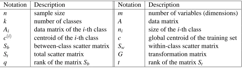
1.3 Notation
For convenience, we present in Table 1 the important notations used in the rest of the paper.
Notation Description Notation Description
n sample size m number of variables (dimensions) k number of classes A data matrix
Ai data matrix of the i-th class ni size of the i-th class
c(i) centroid of the i-th class c global centroid of the training set Sb between-class scatter matrix Sw within-class scatter matrix
St total scatter matrix G transformation matrix
q rank of the matrix Sb t rank of the matrix St
Table 1: Important notations used in the paper
2. Classical Discriminant Analysis
Given a data matrix A∈IRm×n, classical linear discriminant analysis computes a linear transfor-mation G∈IRm×` that maps each column ai of A in the m-dimensional space to a vector yi in the
`-dimensional space:
G : ai∈IRm→yi=GTai∈IR`(` <m).
Assume the original data is already clustered and ordering is imposed on the samples based on cluster membership. The goal of classical LDA is to find a transformation G such that the cluster structure of the original high-dimensional space is preserved in the reduced-dimensional space. Let the data matrix A be partitioned into k classes as A= [A1,···,Ak], where Ai∈IRm×ni, and∑ki=1ni=n.
In discriminant analysis (Fukunaga, 1990), three scatter matrices, called within-class, between-class and total scatter matrices are defined as follows:
Sw =
1 n
k
∑
i=1x
∑
∈Ai(x−c(i))(x−c(i))T,
Sb =
1 n
k
∑
i=1x
∑
∈Ai(c(i)−c)(c(i)−c)T =1
n
k
∑
i=1
ni(c(i)−c)(c(i)−c)T,
St =
1 n
n
∑
j=1
where the centroid c(i)of the i-th class is defined as c(i)= 1
niAie(i)with
e(i)= (1,1,···,1)T ∈IRni,
and the global centroid c is defined as c=1
nAe with
e= (1,1,···,1)T ∈IRn.
It is easy to verify that St=Sb+Sw.
Define the matrices
Hw =
1
√n[A1−c(1)(e(1))T,···,Ak−c(k)(e(k))T],
Hb =
1 √
n[ √n
1(c(1)−c),···,√nk(c(k)−c)],
Ht =
1 √
n(A−ce
T). (2)
Then Sw, Sb, and St can be expressed as
Sw=HwHwT, Sb=HbHbT, St=HtHtT.
The traces of the two scatter matrices Swand Sbcan be computed as follows:
trace(Sw) =
1 n
k
∑
i=1x
∑
∈Ai(x−c(i))T(x−c(i)) =1 n
k
∑
i=1x
∑
∈Ai||x−c(i)||2
trace(Sb) =
1 n
k
∑
i=1
ni(c(i)−c)T(c(i)−c) =
1 n
k
∑
i=1
ni||c(i)−c||2. (3)
Hence, trace(Sw)measures the within-class cohesion, while trace(Sb)measures the between-class
separation.
In the lower-dimensional space resulting from the linear transformation G, the scatter matrices become
SLw=GTSwG, SLb=GTSbG, SLt =GTStG. (4)
An optimal transformation G would maximize trace(SLb) and minimize trace(SLw) simultane-ously, which is equivalent to maximizing trace(SLb)and minimizing trace(SLt)simultaneously, since SL
t =SLw+SLb. A common optimization in classical discriminant analysis (Fukunaga, 1990) is
G=arg max
G
trace((SLt)−1SbL) . (5) The optimization problem in Eq. (5) is equivalent to finding all the eigenvectors that satisfy Sbx=λStx, for λ6=0 (Fukunaga, 1990). The solution can be obtained by applying an
eigen-decomposition on the matrix St−1Sb, if St is nonsingular. There are at most k−1 eigenvectors
corresponding to nonzero eigenvalues, since the rank of the matrix Sb is bounded from above by
Assuming normal distribution for each class with the common covariance matrix, classification based on maximum likelihood estimation results in a nearest class centroid rule, where the distance is measured in terms of the within-class Mahalanobis distance (Hastie et al., 2001). Assuming equal prior for all classes for simplicity, a test point h is classified as class j if
(h−c(j))TSw−1(h−c(j)) (6) is minimized over j=1,···,k. It was shown in (Hastie et al., 1995) that
arg min
j {(h−c
(j))TS−1
w (h−c(j))}=arg minj {||GT(h−c(j))||2}, (7)
where G is the optimal transformation solving the optimization problem in Eq. (5). Thus, clas-sical LDA is equivalent to maximum likelihood classification assuming normal distribution for each class with the common covariance matrix. When the dimension m is much larger than the number of classes k, classification using the reduced representation, i.e., classification based on arg minj{GT(h−c(j))}may give considerable savings (Hastie et al., 1995).
Although relying on heavy assumptions which are not true in many applications, LDA has been proven to be effective. This is mainly due to the fact that a simple, linear model is more robust against noise, and most likely will not overfit. Generalization of LDA by fitting Gaussian mixtures to each class has been studied in (Hastie and Tibshirani, 1996).
Note that classical discriminant analysis requires the total scatter matrix St to be nonsingular,
which may not hold for undersampled data. Several extensions, including two-stage PCA+LDA, Regularized LDA, Penalized LDA, Pseudo-inverse LDA, and LDA/GSVD were proposed in the past to deal with the singularity problems as follows.
A common way to deal with the singularity problems is to apply an intermediate dimension reduction stage such as PCA to reduce the dimension of the original data before classical LDA is applied. The algorithm is known as PCA+LDA (Belhumeur et al., 1997; Swets and Weng, 1996; Zhao et al., 1999). In this two-stage PCA+LDA algorithm, the discriminant stage is preceded by a dimension reduction stage using PCA. The dimension of the subspace transformed by PCA is chosen such as the “reduced” total scatter matrix in the subspace is nonsingular, so that classical LDA can be applied. A limitation of this approach is that the optimal value of the reduced dimension for PCA is difficult to determine. Moreover, the PCA stage may lose some useful information for discrimination.
A simple way to deal with the singularity of St is to apply the idea of regularization, by adding
some constant values to the diagonal elements of St, as St+µIm, for some µ>0, where Im is
an identity matrix. It is easy to verify that St+µIm is positive definite, hence nonsingular. This
approach is called Regularized LDA, or RLDA in short (Friedman, 1989). Regularization is a key in the theory of splines (Wahba, 1998) and is used widely in machine learning, such as Support Vector Machines (SVM) (Vapnik, 1998). It is evident that when µ→∞, we lose the information on St, while very small values of µ may not be sufficiently effective. Cross-validation is commonly
applied for estimating the optimal µ. More recent studies on RLDA can be found in (Dai and Yuen, 2003; Krzanowski et al., 1995).
The Penalized LDA (PLDA) is more general than Regularized LDA. PLDA penalizes the within-class scatter matrix as Sw+Ω, for some penalty matrixΩ.Ωis symmetric and positive semidefinite.
Pseudo-inverse is commonly applied to deal with the singularity problems, which is equivalent to approximating the solution using a least-squares solution method. The use of pseudo-inverse in discriminant analysis has been studied in the past. The Pseudo Fisher Linear Discriminant (PFLDA) (Fukunaga, 1990; Raudys and Duin, 1998; Skurichina and Duin, 1996, 1999) is based on the pseudo-inverse of the scatter matrices. The generalization error of PFLDA was studied in (Skurichina and Duin, 1996), when the size and dimension of the training data vary. Pseudo-inverses of the scatter matrices were also studied in (Krzanowski et al., 1995). Experiments in (Krzanowski et al., 1995) showed that the pseudo-inverse based methods are competitive with RLDA and PCA+LDA.
The LDA/GSVD algorithm (Howland et al., 2003; Ye et al., 2004b) is a more recent approach. The main technique applied is the Generalized Singular Value Decomposition (GSVD) (Golub and Loan, 1996). The criterion F0used in (Ye et al., 2004b) is:
F0(G) =trace (SLb)+SwL
, (8)
where (SLb)+ denotes the pseudo-inverse of the between-class scatter matrix. The definition of pseudo-inverse, as well as its computation via SVD, can be found in Appendix A.
LDA/GSVD aims to find the optimal transformation G that minimizes F0(G), subject to the con-straint that rank(GTHb) =q, where q is the rank of Sb. The above constraint is enforced to preserve
the dimension of the spaces spanned by the centroids in the original and transformed spaces. The optimal solution can be obtained by applying the GSVD. One limitation of this method is the high computational cost of GSVD, especially for large and high-dimensional data sets.
An overview of LDA on undersampled problems can be found in (Krzanowski et al., 1995). The current paper focuses on linear discriminant analysis, which applies linear decision bound-ary. Discriminant analysis can also be studied in the non-linear fashion, so-called kernel discrim-inant analysis, by using the kernel trick (Sch¨okopf and Smola, 2002). It is desirable if the data has weak linear separability. The interested readers can find more details on kernel discriminant analysis in (Baudat and Anouar, 2000; Hand, 1982; Lu et al., 2003; Sch¨okopf and Smola, 2002).
3. Generalization of Discriminant Analysis
Classical discriminant analysis solves an eigen-decomposition problem when St is nonsingular. For
undersampled problems, St is singular, since the sample size n may be smaller than its dimension
m. In this section, we define a new criterion F1, where the nonsingularity of St is not required.
The new criterion F1is a natural extension of the classical one in Eq. (5), where the inverse of a matrix is replaced by the pseudo-inverse (Golub and Loan, 1996). While the inverse of a matrix may not exist, the pseudo-inverse of any matrix is well defined. Moreover, when the matrix is invertible, its pseudo-inverse coincides with its inverse.
The new criterion F1is defined as
F1(G) =trace (SLt)+SLb
. (9)
The optimal transformation matrix G is computed so that F1(G) is maximized. Note that in the following, the matrix G in F1(G)may be omitted if it is clear from the content.
3.1 Simultaneous Diagonalization of Scatter Matrices
In this section, we take a closer look at the relationship among three scatter matrices Sb, Sw, and St,
and show how to diagonalize them simultaneously.
Let Ht =UΣVT be the SVD of Ht, where Ht is defined in Eq. (2), U and V are orthogonal,
Σ= Σ
t 0
0 0
,Σt∈IRt×t is diagonal, and t =rank(St). Then
St =HtHtT =UΣVTVΣTUT=UΣΣTUT =U
Σ2
t 0
0 0
UT. (10)
Let U = (U1,U2) be a partition of U , such that U1∈IRm×t and U2∈IRm×(m−t). Since St =
Sb+Sw, we have
Σ2
t 0
0 0
= UT(Sb+Sw)U
=
U1T U2T
Sb(U1,U2) +
U1T U2T
Sw(U1,U2) =
U1TSbU1 U1TSbU2 U2TSbU1 U2TSbU2
+
U1TSwU1 U1TSwU2 U2TSwU1 U2TSwU2
. (11)
It follows that U2TSbU2+U2TSwU2=0. Therefore, U2TSbU2=0 and U2TSwU2=0, since both are positive semidefinite. We thus have U1TSbU2=0 and U1TSwU2=0, since both matrices on the right hand size of Eq. (11) are positive semidefinite. That is,
UTSbU=
U1TSbU1 0
0 0
, UTSwU=
U1TSwU1 0
0 0
. (12)
From Eq. (11) and Eq. (12), we haveΣ2t =U1TSbU1+U1TSwU1. It follows that
It =Σt−1U1TSbU1Σ−t 1+Σ−t 1U1TSwU1Σ−t 1. (13)
Denote B=Σ−t 1U1THb and let B=P ˜ΣQT be the SVD of B, where P and Q are orthogonal and ˜
Σis diagonal. Then
Σ−1
t U1TSbU1Σ−t 1=P ˜Σ2PT =PΣbPT,
where
Σb≡Σ˜2=diag(λ1,···,λt),
λ1≥ ··· ≥λq>0=λq+1=···=λt,
and q=rank(Sb).
It follows from Eq. (13) that
It=Σb+PTΣ−t 1U1TSwU1Σ−t 1P.
Hence
PTΣt−1U1TSwU1Σ−t 1P=It−Σb≡Σw
Combining all these together, we have
XTSbX=
Σ
b 0
0 0
≡Db, XTSwX=
Σ
w 0
0 0
≡Dw, XTStX=
It 0
0 0
≡Dt, (14)
where
X=U Σ−1
t P 0
0 I
. (15)
In summary, the matrix X in Eq. (15) simultaneously diagonalizes Sb, Sw, and St.
3.2 Maximization of the F1Criterion
In this section, we derive the generalized discriminant analysis by maximizing the F1criterion de-fined in Eq. (9). The main technique applied is the simultaneous diagonalization of scatter matrices from last section. We show in this section that the solutions to the proposed criterion F1 can be characterized as G=XqM, where Xqis the matrix consisting of the first q columns of X , defined in
Eq. (15), q=rank(Sb), and M∈IRq×qis an arbitrary nonsingular matrix.
We first present two lemmas. The proof of Lemma 3.1 is straightforward from standard linear algebra and a generalization of Lemma 3.2 can be found in (Edelman et al., 1998).
Lemma 3.1 For any matrix A∈IRm×n, the following equality holds:(ATA)+=A+(A+)T.
Lemma 3.2 Let A∈IRm×mbe symmetric and positive semidefinite and let xibe the eigenvector of A
corresponding to the i-th largest eigenvalueλi. Then, for any M∈IRm×s(s≤m)with orthonormal
columns, the following inequality holds,
trace MTAM
≤λ1+···+λs,
where the equality holds if M= [x1,···,xs]Q, for any orthogonal matrix Q∈IRs×s.
The main result of this section is summarized in the following theorem.
Theorem 3.1 Let X be the matrix defined in Eq. (15) and Xqbe the matrix consisting of the first q
columns of X , where q=rank(Sb). Then G=XqM, for any nonsingular M, maximizes F1 defined in Eq. (9).
Proof By the simultaneous diagonalization of the three scatter matrices in Eq. (14), we have
SLb = GTSbG=GT(X−1)T(XTSbX)X−1G=G˜TDbG˜,
SLt = GTStG=GT(X−1)T(XTStX)X−1G=G˜TDtG˜, (16)
where ˜G=X−1G. Let ˜G=
G1 G2
be a partition of ˜G so that G1∈IRt×`and G2∈IR(m−t)×`. It follows that SbL=G˜TD
bG˜ =GT1ΣbG1, StL=G˜TDtG˜ =GT1G1. Hence
F1=trace (GT1G1)+(GT1ΣbG1)
=trace (G1G+1)
TΣ
b(G1G+1)
where the second equality follows from Lemma 3.1.
Recall that Σb =diag(λ1,···,λt), where λ1 ≥ ··· ≥ λq >0=λq+1 =···=λt. Let G1 = R
Σ
δ 0
0 0
ST be the SVD of G1, where R and S are orthogonal,Σδis diagonal, andδ=rank(G1). Then G+1 =S
Σ−1
δ 0
0 0
RT, and G1G+1 =R
Iδ 0 0 0
RT. It follows that
F1 = trace (G1G+1)
TΣ
b(G1G+1)
=trace
R
Iδ 0 0 0
RTΣbR
Iδ 0
0 0 RT = trace
Iδ 0 0 0
RTΣbR
Iδ 0
0 0
=trace RTδΣbRδ
≤λ1+···+λq.
where Rδis the matrix consisting of the firstδcolumns of R, and the last inequality follows from
Lemma 3.2. By Lemma 3.2 again, the above inequality becomes equality, if Rδ=
W 0
, for any
orthogonal W∈IRq×q,δ=q, and`=q. Under this choice of Rδ,
G1=RqΣqST=
WΣqST
0
.
We observe that the maximization of F1is independent of G2, and simply set it to zero. Therefore, the maximum of F1is attained when
˜ G= G1 G2 =
WΣqST
0
.
Note that the orthogonal matrices W and S, and the diagonal matrix Σq are arbitrary. Hence,
M=WΣqST is an arbitrary nonsingular matrix. It follows that G=X ˜G=XqM, for any nonsingular
M, maximizes F1. This completes the proof of the theorem.
Remark 1 Note that it is in general not true that F1(H) =F1(HM), for any nonsingular M. How-ever, Theorem 3.1 implies that for H=Xq, we have F1(H) =F1(HM), for any nonsingular M. 4. Uncorrelated LDA Versus Orthogonal LDA
From last section, G=XqM, for any nonsingular M maximizes the F1criterion. A natural question is: How to choose the best M? In this section, we consider two specific choices of M, which lead to two distinct algorithms: Uncorrelated LDA and Orthogonal LDA.
4.1 Uncorrelated LDA
The simplest choice of M is the identity matrix, i.e., M=Iq. That is, G=Xq. It follows that
XT
qStXq=Iq, i.e., the columns of the transformation G are St-orthogonal. Recall that two vectors x
and y are St-orthogonal, if xTSty=0. The solution corresponds to the Uncorrelated LDA, originally
Algorithm 1: Uncorrelated LDA Input: data matrix A
Output: transformation matrix G
1. Form three matrices Hb, Hw, and Ht as in Eq. (2);
2. Compute reduced SVD of Ht as Ht=U1ΣtV1T;
3. B←Σt−1U1THb;
4. Compute SVD of B as B=PΣQT; q←rank(B); 5. X ←U1Σt−1P;
6. G←Xq;
ULDA was originally proposed to compute the optimal discriminant vectors that are St-orthogonal.
Specifically, suppose r vectorsφ1,φ2,···,φrare obtained, then the(r+1)-th vectorφr+1of ULDA is the one that maximizes the Fisher criterion function
f(φ) = φ
TS bφ
φTS wφ
, (17)
subject to the constraints:
φT
r+1Stφi=0, i=1,···,r.
The algorithm in (Jin et al., 2001a) finds φi successively as follows: The j-th discriminant
vectorφj of ULDA is the eigenvector corresponding to the maximum eigenvalue of the following
generalized eigenvalue problem:
UjSbφj=λjSwφj,
where
U1 = Im,
Uj = Im−StDTj(DjStS−w1StDTj)−1DjStS−w1(j>1),
Dj = [φ1,···,φj−1]T(j>1), and Imis the identity matrix.
A key property of ULDA is that the features in the reduced space are uncorrelated to each other, as stated in the following proposition.
Proposition 4.1 Let the transformation matrix for ULDA be G= [g1,···,gd], for some d>0. The
original feature vector A is transformed into Z=GTA, where the i-th feature component of Z is Zi=gTi A. Assume that gi and gj are St-orthogonal to each other, i.e., gTi Stgj=0, for i6= j. Then
the correlation between Ziand Zjis 0, for i6= j. That is, Ziand Zjare uncorrelated to each other.
Proof The covariance between Ziand Zj can be computed as
Cov(Zi,Zj) =E(Zi−EZi)(Zj−EZj) =gTi {E(A−EA)(A−EA)T}gj=gTi Stgj. (18)
Hence, their correlation coefficient is
Cor(Zi,Zj) =
gTi Stgj
q gTi Stgi
q gTjStgj
Since gTi Stgj=0, for i6= j, we have Cor(Zi,Zj) =0, for i6= j. This completes the proof of the
proposition.
In (Ye et al., 2004a), an efficient algorithm for ULDA was proposed, based on the following optimization problem:
G=arg max
G {trac((S L
t +µI`)−1SLb)}. (20)
Note that SLt +µI` is always nonsingular for µ>0, since StLis positive semidefinite. One key
result in (Ye et al., 2004a) shows that the optimal transformation G solving the optimization problem in Eq. (20) is independent of µ.
Interestingly, it can be shown that G=Xqsolves the optimization problem in Eq. (20) as stated
in the following proposition. Detailed proof follows the one in (Ye et al., 2004a) and is thus omitted.
Proposition 4.2 Let G=Xq, where Xqis the matrix consisting of the first q columns of X , and X is
defined in Eq. (15). Then G solves the optimization problem in Eq. (20).
4.1.1 RELATIONSHIPBETWEENULDAAND THEEIGEN-DECOMPOSITION OFS+t Sb
In this section, we study the relationship between ULDA and the eigen-decomposition of S+t Sb.
More specifically, we show that the discriminant vectors of ULDA are eigenvectors of St+Sb
cor-responding to nonzero eigenvalues. Recall that classical LDA computes the optimal discriminant vectors by solving an eigenvalue problem on S−t 1Sb, assuming St is nonsingular (See Section 2).
This equivalence result shows that ULDA is a natural extension of classical LDA by replacing in-verse with pseudo-inin-verse, when dealing with singular St.
From Eq. (14), we have XTStX=Dt, where
X=U Σ−1
t P 0
0 0
, and Dt =
It 0
0 0
.
Note that P is orthogonal. It follows that
St =X−TDtX−1=U
Σ
tP 0
0 0
It 0
0 0
PTΣ t 0
0 0
UT =U Σ2
t 0
0 0
UT,
Hence,
S+t =U
Σ−2
t 0
0 0
UT.
It is easy to verify that
X DtXT =U
Σ−2
t 0
0 0
UT.
It follows that
St+=X DtXT, (21)
and
St+Sb= X DtXT
X−1DbX−1
=X DtDbX−1.
Therefore, the columns of Xqform the eigenvectors of S+t Sbcorresponding to nonzero eigenvalues,
Algorithm 2: Orthogonal LDA Input: data matrix A
Output: transformation matrix G
1. Compute the matrix Xqas in ULDA (Steps 1–5 of Algorithm 1);
2. Compute QR decomposition of Xqas Xq=Q ˜˜R;
3. G←Q;˜
4.2 Orthogonal LDA
LDA with orthogonal discriminant vectors is a natural alternative to ULDA. Let Xq=Q ˜˜R be the QR
decomposition of Xq, then we can simply choose M=R˜−1so that the columns of G=XqM=Q are˜
orthogonal to each other. The pseudo-code for OLDA is given in Algorithm 2.
Note that in the literature of LDA, Foley-Sammon LDA (FSLDA) is also known for its orthogo-nal discriminant vectors. FSLDA was first proposed by Foley and Sammon for two-class problems (Foley and Sammon, 1975). It was then extended to the multi-class problems by Duchene and Leclercq (Duchene and Leclerq, 1988). Specifically, suppose r vectorsφ1,φ2,···,φr are obtained,
then the(r+1)-th vectorφr+1 of FSLDA is the one that maximizes the Fisher criterion function f(φ)defined in Eq. (17), subject to the constraints:φTr+1φi=0, i=1,···,r.
The algorithm in (Duchene and Leclerq, 1988) findsφi successively as follows: The j-th
dis-criminant vectorφjof FSLDA is the eigenvector corresponding to the maximum eigenvalue of the
following matrix:
Im−S−w1DTjS−j1Dj
Sw−1Sb,
where
Dj= [φ1,···,φj−1]T(j>1),and Sj=DjS−w1DTj.
The above FSLDA algorithm may be expensive for large and high-dimensional data sets. More details on the computation of FSLDA can be found in (Duchene and Leclerq, 1988).
It is worthwhile to point out that both ULDA and FSLDA use the same Fisher criterion func-tion, and the main difference is that the optimal discriminant vectors generated by ULDA are St
-orthogonal to each other, while the optimal discriminant vectors of FSLDA are -orthogonal to each other.
The common point of the proposed OLDA algorithm and the FSLDA algorithm described above is that the transformation matrix has orthogonal columns. However, these two algorithms were derived from distinct perspectives.
4.3 Discussions
As discussed in Section 2, classical LDA is equivalent to maximum likelihood classification as-suming normal distribution for each class with the common covariance matrix. Classification in classical LDA based on the maximum likelihood estimation is based on the Mahalanobis distance as follows: a test point h is classified as class j if
j=arg min
j (h−c
(j))TS−1
which is equivalent to
j=arg min
j (h−c
(j))TS−1
t (h−c(j)). (23)
We show in the following that the classification in ULDA uses the following distance:
(h−c(j))TSt+(h−c(j)). (24)
The main result is summarized in the following theorem.
Theorem 4.1 Let G be the optimal transformation matrix for ULDA, and let h be any test point. Then
arg min
j
n
(h−c(j))TSt+(h−c(j))o=arg min
j
n
||GT(h−c(j))||2o.
Proof Let Xi be the i-th column of X . From Eq. (21), we have
St+=X DtXT = t
∑
i=1
XiXiT=GGT+ t
∑
i=q+1 XiXiT,
where G consists of the first q columns of X , and q=rank(Sb).
Recall from Section 3.1 that X diagonalizes Sb and XiTSbXi =0, for i=q+1,···,t. Hence
HbXi=0, or(c(j))TXi=cXi, for all j=1,···,k. It follows that
(h−c(j))TSt+(h−c(j)) = (h−c(j))TGGT(h−c(j)) +
t
∑
i=q+1
(h−c(j))TXiXiT(h−c(j))
= ||GT(h−c(j))||2+
t
∑
i=q+1
(h−c)TXiXiT(h−c). (25)
The second term on the right hand side of Eq. (25) is independent of class j, hence
arg min
j
n
(h−c(j))TS+
t (h−c(j))
o
=arg min
j
n
||GT(h−c(j))||2o. This completes the proof of the theorem.
Theorem 4.1 shows that the classification rule in ULDA is a variant of the one used in classical LDA. ULDA can be considered as an extension of classical LDA for singular scatter matrices. The result does not extend to OLDA. However, with whitened total scatter matrix, that is if St is an
identity matrix, OLDA is equivalent to ULDA.
Geometrically, both ULDA and OLDA project the data onto the subspace spanned by the cen-troids. ULDA removes the correlation among the features in the transformed space, which is theo-retically sound but may be sensitive to the noise in the data. On the other hand, OLDA applies or-thogonal transformation ˜Q, by factoring out the ˜R matrix through the QR decomposition of Xq=Q ˜˜R.
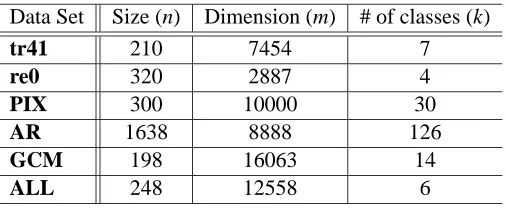
Data Set Size (n) Dimension (m) # of classes (k)
tr41 210 7454 7
re0 320 2887 4
PIX 300 10000 30
AR 1638 8888 126
GCM 198 16063 14
ALL 248 12558 6
Table 2: Statistics for our test data sets
5. Experiments
We divide the experiments into three parts. Section 5.1 describes our test data sets. Section 5.2 evaluates ULDA and OLDA in terms of classification accuracy. We study the effect of the matrix M in Section 5.3. Recall that G=XqM, for any nonsingular M maximizes the F1criterion.
Both ULDA and OLDA were implemented in MATLAB and the source codes may be accessed at http://www.cs.umn.edu/∼jieping/UOLDA.
5.1 Data Sets
We have three types of data for the evaluation: text documents, including tr41 and re0; face im-ages, including PIX and AR; and gene expression data, including GCM and ALL. The important statistics of these data sets are summarized as follows (see also Table 2):
• tr41 is a text document data set, derived from the TREC-5, TREC-6, and TREC-7 collections (TREC, 1999). It includes 210 documents belonging to 7 different classes. The dimension of this data set is 7454.
• re0 is another text document data set, derived from Reuters-21578 text categorization test collection Distribution 1.0 (Lewis, 1999). It includes 320 documents belonging to 4 different classes. The dimension of this data set is 2887.
• PIX1is a face image data set, which contains 300 face images of 30 persons. The size of PIX images is 512×512. We subsample the images down to a size of 100×100=10000.
• AR2(Martinez and Benavente, 1998), is a large face image data set. The instance of each face may contain pretty large areas of occlusion, due to the presence of sun glasses and scarves. We use a subset of AR. This subset contains 1638 face images of 126 individuals. Its image size is 768×576. We first crop the image from row 100 to 500, and column 200 to 550, and then subsample the cropped images down to a size of 101×88=8888.
• GCM is a gene expression data set consisting of 198 human tumor samples spanning fourteen different cancer types. The data set was first studied in (Ramaswamy and et al., 2001; Yeang and et al., 2001). The breakdown of the sample classes is as follows: 12 breast samples, 14
1. http://peipa.essex.ac.uk/ipa/pix/faces/manchester/test-hard/
prostate samples, 12 lung samples, 12 colorectal samples, 22 lymphoma samples, 11 bladder samples, 10 melanoma samples, 10 uterus samples, 30 leukemia samples, 11 renal samples, 11 pancreas samples, 12 ovary samples, 11 mesothelioma samples, and 20 CNS samples.
• ALL3is another gene expression data set consisting of six diagnostic groups (Yeoh and et al., 2002). The breakdown of the samples is: 15 samples for BCR, 27 samples for E2A, 64 samples for Hyperdip, 20 samples for MLL, 43 samples for T, and 79 samples for TEL.
5.2 Comparison on Classification Accuracy
In this experiment, we evaluate ULDA and OLDA in terms of classification accuracy. For the GCM and ALL gene expression data sets, the test sets were provided. In the absence of original test sets, such as the two document data sets and the two face image data sets, we perform our comparative study by repeated random splitting into training and test sets exactly as in (Dudoit et al., 2002). The data were randomly partitioned into a training set consisting of two-thirds of the whole set and a test set consisting of one-third of the whole set. To reduce the variability, the splitting was repeated 50 times and the resulting accuracies were averaged. Note that during each run, dimension reduction is applied to the training set only. For RLDA, the results depend on the choice of the parameter µ. We choose the best µ through cross-validation. The range for µ is between 0.001 and 10.
The results of the three algorithms on the six data sets are presented in Table 3. The main observation from Table 3 is that OLDA is competitive with ULDA and RLDA in all six data sets. We also observe that in most cases, RLDA outperforms ULDA and is competitive with OLDA.
It is interesting to note that OLDA achieves higher accuracies than ULDA for the two face image data sets and two gene expression data sets, while it achieves accuracies close to those of ULDA for the two text document data sets. For the GCM gene expression data set, OLDA achieved classification accuracy 3% higher than that of OLDA. This may be related to the effect of the noise removal inherent in OLDA as discussed in Section 4.3.
5.3 Effect of the Matrix M
In this experiment, we study the effect of the matrix M on classification using the GCM and ALL data sets. Recall that the solution to the proposed criterion is G=XqM, for any nonsingular M. Two
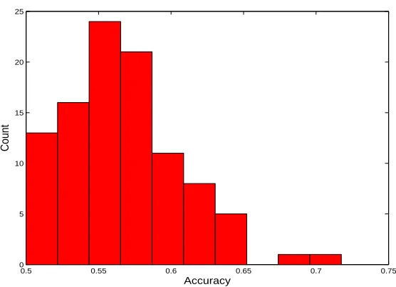
specific choices of M were studied, which correspond to ULDA and OLDA. In this experiment, we randomly generated 100 matrices for M and computed the accuracies using the corresponding transformation matrices. Figure 1 shows the histogram of the resulting accuracies on GCM, where the x-axis represents the range of resulting accuracies (divided into small intervals), and the y-axis represents the number (count) for each interval. The main observations are:
• None of the accuracies is higher than those of ULDA (73.91%) and OLDA (76.09%). ULDA and OLDA are probably two of the best ones among the family of solutions to the proposed criterion.
• In Figure 1, most of the accuracies are around 55%, which is much lower than those of ULDA and OLDA. Thus, the choice of M does make a big difference. Among the family of solutions to the proposed criterion, most of them perform quite poorly in comparison to ULDA and OLDA.
Data Set Accuracy
ULDA OLDA RLDA
tr41 96.69±1.90 96.34±2.10 96.23±2.17 re0 86.26±2.46 86.13±2.58 87.34±2.37 PIX 96.16±2.48 98.00±1.66 96.31±2.20 AR 90.94±0.96 92.77±1.04 91.11±1.02
GCM 73.91 76.09 78.26
ALL 98.82 100.0 98.82
Table 3: Comparison of classification accuracy and standard deviation of three algorithms: ULDA (Uncorrelated LDA), OLDA (Orthogonal LDA), and RLDA (Regularized LDA), on the six data sets. The mean and standard deviation of accuracies from fifty runs are reported for tr41, re0, PIX, and AR. Note that for the two gene expression data sets: GCM and ALL, we use the original test sets. Thus the standard deviation for these two data sets are not reported.
0.5 0.55 0.6 0.65 0.7 0.75
0 5 10 15 20 25
Accuracy
Count
Figure 1: Effect of the matrix M using the GCM data set. The corresponding accuracies of ULDA and OLDA are 73.91% and 76.09%, respectively.
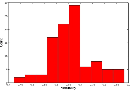
The result on ALL is shown in Figure 2. We can observe the same trend as in GCM, that is, most of the accuracies are much lower than those of ULDA and OLDA.
6. Conclusions and Future Directions
0.4 0.45 0.5 0.55 0.6 0.65 0.7 0.75 0.8 0.85 0.9 0
5 10 15 20 25 30
Accuracy
Count
Figure 2: Effect of the matrix M using the ALL data set. The corresponding accuracies of ULDA and OLDA are 98.82% and 100.0%, respectively.
is applicable regardless of the relative sizes of the data dimension and sample size, overcoming a limitation of the classical LDA. A detailed mathematical derivation for the proposed optimization problem is presented. It is based on the simultaneous diagonalization of the three scatter matrices.
The solutions to the proposed criterion form a family of algorithms for generalized LDA, which can be characterized in a closed form. Among the family of solutions, we study two specific ones, namely ULDA and OLDA, where ULDA was previously proposed for feature extraction and di-mension reduction and OLDA is a novel algorithm. ULDA has the property that the features in the reduced space are uncorrelated, while OLDA has the property that the discriminant vectors obtained are orthogonal to each other. Experiment on a variety of real-world data sets show that OLDA is competitive with ULDA and RLDA in terms of classification accuracy.
In this paper, we focus on two specific algorithms, ULDA and OLDA, for generalized LDA. A promising direction is to find algorithms with sparse transformation matrices. Sparsity has re-cently received much attention for extending Principal Component Analysis (d’Aspremont et al., 2004; Jolliffe and Uddin, 2003). One of our future work is to incorporate the sparsity criterion in discriminant analysis.
Acknowledgments
Appendix A.
The pseudo-inverse of a matrix is defined as follows.
Definition 2 The pseudo-inverse of a matrix A, denoted as A+, refers to the unique matrix satisfying the following four conditions:
(1)A+AA+=A+, (2)AA+A=A, (3) (AA+)T =AA+, (4)(A+A)T=A+A.
The pseudo-inverse is commonly computed by the SVD as follows (Golub and Loan, 1996).
Let A=U Σ
0 0 0
VT be the SVD of A, where U and V are orthogonal andΣis diagonal with
positive diagonal entries. Then, A+=V Σ−1
0 0 0
UT.
References
G. Baudat and F. Anouar. Generalized discriminant analysis using a kernel approach. Neural Computation, 12(10):2385–2404, 2000.
P. N. Belhumeur, J. P. Hespanha, and D. J. Kriegman. Eigenfaces vs. Fisherfaces: Recognition using class specific linear projection. IEEE Transactions on Pattern Analysis and Machine Intelligence, 19(7):711–720, 1997.
M. W. Berry, S. T. Dumais, and G. W. O’Brie. Using linear algebra for intelligent information retrieval. SIAM Review, 37:573–595, 1995.
D. Q. Dai and P. C. Yuen. Regularized discriminant analysis and its application to face recognition. Pattern Recognition, 36:845–847, 2003.
A. d’Aspremont, L. Ghaoui, M. I. Jordan, and G. R. G. Lanckriet. A direct formulation for sparse PCA using semidefinite programming. In Proceedings of the Eighteenth Annual Conference on Advances in Neural Information Processing Systems, 2004.
S. Deerwester, S. T. Dumais, G. W. Furnas, T. K. Landauer, and R. Harshman. Indexing by latent semantic analysis. Journal of the Society for Information Scienc, 41:391–407, 1990.
L. Duchene and S. Leclerq. An optimal transformation for discriminant and principal component analysis. IEEE Transactions on Pattern Analysis and Machine Intelligence, 10(6):978–983, 1988.
R. O. Duda, P. E. Hart, and D. Stork. Pattern Classification. Wiley, 2000.
S. Dudoit, J. Fridlyand, and T. P. Speed. Comparison of discrimination methods for the classification of tumors using gene expression data. Journal of the American Statistical Association, 97(457): 77–87, 2002.
A. Edelman, T. A. Arias, and S. T. Smith. The geometry of algorithms with orthogonality con-straints. SIAM Journal on Matrix Analysis and Applications, 20(2):303–353, 1998.
J. H. Friedman. Regularized discriminant analysis. Journal of the American Statistical Association, 84(405):165–175, 1989.
K. Fukunaga. Introduction to Statistical Pattern Classification. Academic Press, USA, 1990.
G. H. Golub and C. F. Van Loan. Matrix Computations. The Johns Hopkins University Press, Baltimore, MD, USA, third edition, 1996.
D. J. Hand. Kernel discriminant analysis. Research Studies Press/Wiley, 1982.
T. Hastie, A. Buja, and R. Tibshirani. Penalized discriminant analysis. Annals of Statistics, 23: 73–102, 1995.
T. Hastie and R. Tibshirani. Discriminant analysis by Gaussian mixtures. Journal of the Royal Statistical Society series B, 58:158–176, 1996.
T. Hastie, R. Tibshirani, and J. H. Friedman. The elements of statistical learning : data mining, inference, and prediction. Springer, 2001.
P. Howland, M. Jeon, and H. Park. Structure preserving dimension reduction for clustered text data based on the generalized singular value decomposition. SIAM Journal on Matrix Analysis and Applications, 25(1):165–179, 2003.
Z. Jin, J. Y. Yang, Z. S. Hu, and Z. Lou. Face recognition based on the uncorrelated discriminant transformation. Pattern Recognition, 34:1405–1416, 2001a.
Z. Jin, J. Y. Yang, Z. M. Tang, and Z. S. Hu. A theorem on the uncorrelated optimal discriminant vectors. Pattern Recognition, 34(10):2041–2047, 2001b.
I. T. Jolliffe and M. Uddin. A modified principal component technique based on the lasso. Journal of Computational and Graphical Statistics, 12:531–547, 2003.
W. J. Krzanowski, P. Jonathan, W. V. McCarthy, and M. R. Thomas. Discriminant analysis with singular covariance matrices: methods and applications to spectroscopic data. Applied Statistics, 44:101–115, 1995.
D. D. Lewis. Reuters-21578 text categorization test collection distribution 1.0. http://
www.research.att.com/∼lewis, 1999.
J. Lu, K. N. Plataniotis, and A. N. Venetsanopoulos. Face recognition using kernel direct discrimi-nant analysis algorithms. IEEE Transactions on Neural Networks, 14(1):117–126, 2003.
A. M. Martinez and R. Benavente. The AR face database. Technical Report No. 24, 1998.
S. Ramaswamy and et al. Multiclass cancer diagnosis using tumor gene expression signatures. Proceedings of the National Academy of Science, 98(26):15149–15154, 2001.
S. Raudys and R. P. W. Duin. On expected classification error of the fisher linear classifier with pseudo-inverse covariance matrix. Pattern Recognition Letters, 19(5-6):385–392, 1998.
M. Skurichina and R. P. W. Duin. Stabilizing classifiers for very small sample size. In Proc. International Conference on Pattern Recognition, pages 891–896, 1996.
M. Skurichina and R. P. W. Duin. Regularization of linear classifiers by adding redundant features. Pattern Analysis and Applications, 2(1):44–52, 1999.
D. L. Swets and J. Weng. Using discriminant eigenfeatures for image retrieval. IEEE Transactions on Pattern Analysis and Machine Intelligence, 18(8):831–836, 1996.
TREC. Text Retrieval conference. http://trec.nist.gov, 1999.
M. A. Turk and A. P. Pentland. Face recognition using Eigenfaces. In IEEE Computer Society Conference on Computer Vision and Pattern Recognition, pages 586–591, 1991.
V. N. Vapnik. Statistical Learning Theory. Wiley, New York, 1998.
G. Wahba. Spline Models for Observational Data. Society for Industrial & Applied Mathematics, 1998.
J. Ye, R. Janardan, Q. Li, and H. Park. Feature extraction via generalized uncorrelated linear dis-criminant analysis. In The Twenty-First International Conference on Machine Learning, pages 895–902, 2004a.
J. Ye, R. Janardan, C. H. Park, and H. Park. An optimization criterion for generalized discrimi-nant analysis on undersampled problems. IEEE Transactions on Pattern Analysis and Machine Intelligence, 26(8):982–994, 2004b.
C. H. Yeang and et al. Molecular classification of multiple tumor types. Bioinformatics, 17(1):1–7, 2001.
E. J. Yeoh and et al. Classification, subtype diswcovery, and prediction of outcome in pediatric lymphoblastic leukemia by gene expression profiling. Cancer Cell, 1(2):133–143, 2002.