Smooth
ε-Insensitive Regression by Loss Symmetrization
Ofer Dekel [email protected]
Shai Shalev-Shwartz [email protected]
Yoram Singer [email protected]
School of Computer Science and Engineering The Hebrew University
Jerusalem, 91904, Israel
Editors:Kristin P. Bennett and Nicol`o Cesa-Bianchi
Abstract
We describe new loss functions for regression problems along with an accompanying al-gorithmic framework which utilizes these functions. These loss functions are derived by symmetrization of margin-based losses commonly used in boosting algorithms, namely, the logistic loss and the exponential loss. The resulting symmetric logistic loss can be viewed as a smooth approximation to the ε-insensitive hinge loss used in support vector regres-sion. We describe and analyze two parametric families of batch learning algorithms for minimizing these symmetric losses. The first family employs an iterativelog-additive up-date which can be viewed as a regression counterpart to recent boosting algorithms. The second family utilizes an iterative additive update step. We also describe and analyze online gradient descent (GD) and exponentiated gradient (EG) algorithms for the sym-metric logistic loss. A byproduct of our work is a new simple form of regularization for boosting-based classification and regression algorithms. Our regression framework also has implications on classification algorithms, namely, a new additive update boosting algorithm for classification. We demonstrate the merits of our algorithms in a series of experiments.
1. Introduction
The focus of this paper is supervised learning of real-valued functions. We observe a se-quence S = {(x1, y1), . . . ,(xm, ym)} of instance-target pairs, where the instances are
vec-tors in Rn and the targets are real-valued scalars, yi ∈R. Our goal is to learn a function
f : Rn → R which provides a good approximation of the target values from their
corre-sponding instance vectors. Such a function is often referred to as a regression function or a regressor for short. Regression problems have long been the focus of research pa-pers in statistics and learning theory (see for instance the book by Hastie, Tibshirani, and Friedman (2001) and the references therein). In this paper we discuss learning of linear
regressors, that is, f is of the form f(x) =λ·x. This setting is also suitable for learning
a linear combination of base regressors of the form f(x) =Pl
j=1λjhj(x) where each base
regressor hj is a mapping from an instance domain X into R. The latter form enables us
to employ kernels by settinghj(x) =K(xj,x).
The class of linear regressors is rather restricted. Furthermore, in real applications both the instances and the target values are often corrupted by noise and a perfect mapping
−5 0 5 0
1 2 3 4 5 6 7 8
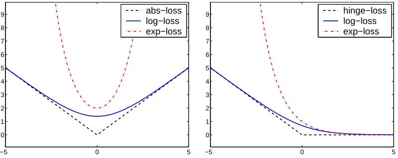
9 abs−loss
log−loss exp−loss
−5 0 5
0 1 2 3 4 5 6 7 8
9 hinge−loss
log−loss exp−loss
Figure 1: Constructing regression losses (left) by symmetrization of margin losses (right).
function L : R×R → R+ which determines the penalty for a discrepancy between the
predicted target, f(x), and the true (observed) target y. As we discuss shortly, the loss
functions we consider in this paper depend only on the discrepancy between the predicted
target and the true target δ =f(x)−y, hence L can be viewed as a function from Rinto
R+. We therefore allow ourselves to overload our notation and denote L(δ) =L(f(x), y).
Given a loss function L, the goal of a regression algorithm is to find a regressorf which
attains a small total loss on the training set S,
Loss(λ, S) =
m
X
i=1
L(f(xi)−yi) = m
X
i=1
L(λ·xi−yi).
Denoting the discrepancyλ·xi−yi byδi, we note that two common approaches to solving
regression problems are to minimize either the sum of the absolute discrepancies over the
sample (P
i|δi|) or the sum of squared discrepancies (
P
iδ2i). It has been argued that the
squared loss is sensitive to outliers, hence robust regression algorithms often employ the
absolute loss (Huber, 1981). Furthermore, it is often the case that the exact discrepancy
between λ·x and y is unimportant so long as it falls below an insensitivity parameter
ε. Formally, the ε-insensitive hinge loss, denoted |δ|ε, is zero if |δ| ≤ ε and is |δ| −ε for
|δ|> ε (see also the left hand side of Figure 2). The ε-insensitive hinge loss is not smooth
as its derivative is discontinuous at δ =±ε. Several batch learning algorithms have been
proposed for minimizing the ε-insensitive hinge loss (see for example Vapnik, 1998; Smola
and Sch¨olkopf, 1998). However, these algorithms are based on rather complex constrained
optimization techniques since the ε-insensitive hinge loss is a non-smooth function.
The first loss function presented in this paper is a smooth approximation to the ε
-insensitive hinge loss. Define thesymmetric ε-insensitive logistic loss, orlog-loss for short,
to be,
Llog(δ;ε) = log
1 +eδ−ε+ log1 +e−δ−ε−κ. (1)
Whenever it is clear from context we omit the insensitivity parameterεand denote this loss
by Llog(δ). The constantκ in Eq. (1) equals 2 log(1 +e−ε) and is set such that Llog(0) = 0.
−15 −10 −5 0 5 10 15 0
1 2 3 4 5 6 7 8
9 |δ|ε
log−loss
−150 −100 −50 0 50 100 150
0 10 20 30 40 50 60 70 80
90 comb−loss
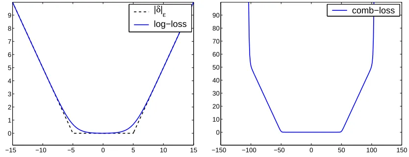
Figure 2: The smoothε-insensitive log-loss (left) and the comb-loss (right).
henceforth. In Figure 2 we depict the ε-insensitive log-loss along with the ε-insensitive
hinge loss for ε= 5. Note that the ε-insensitive log-loss provides a smooth upper bound
on the ε-insensitive hinge loss. Moreover, note that for this particular choice of ε and for
|δ|<2 and|δ|>8 the log-loss and hinge-loss are graphically indistinguishable.
To motivate our construction, let us take a short detour and discuss a recent view of margin-based classification algorithms. In the binary classification setting discussed in Friedman et al. (2000), Collins et al. (2002) and Lebanon and Lafferty (2001), we are
provided with instance-label pairs, (x, y), where, in contrast to regression, each label takes
one of two values, namelyy∈ {−1,+1}. A real-valued classifier is a functionf into the reals
such that sign(f(x)) is the predicted label and |f(x)| is the confidence of f in its
predic-tion. The productyf(x) is called the (signed) margin of the instance-label pair (x, y). The
goal of a margin-based classifier is to attain large margin values on as many instances as possible. Learning algorithms for margin-based classifiers typically employ a margin-based
loss functionLc(yf(x)) and attempt to minimize the total loss over all instances in a given
sample. One of the margin losses discussed is the logistic loss, which takes the form
Lc(yf(x)) = log1 +e−yf(x). (2)
We discuss a general technique for reducing a regression problem to a margin-based
clas-sification problem called loss symmetrization. The symmetric log-loss given in Eq. (1) is
obtained by applying this technique to the classification logistic loss in Eq. (2). The tech-nique of loss symmetrization was previously discussed in Bi and Bennett (2003) in the context of support vector regression.
Formally, let [u;v] denote the concatenation of an additional elementv to the end of a
vectoru. We replace every instance-targetpair (x, y) from the regression problem withtwo
classification instance-label pairs,
(x, y) 7→
([x;−y+ε],+1) ([x;−y−ε],−1) .
−y +ε to the first newly created instance and set its label to +1. Symmetrically, we
concatenate −y−εto the second copy of the instance and set its label to −1. We define
the linear classifierto be the vector [λ; 1]∈Rn+1. It is simple to verify that,
Llog(λ·x−y;ε) =Lc([λ; 1]·[x;−y+ε]) +Lc(−[λ; 1]·[x;−y−ε]).
In Figure 1 we give an illustration of the above construction. We have thus reduced a
regression problem of m instances in Rn with targets in Rto a classification problem with
2m instances inRn+1 and binary labels in {±1}.
The work in Collins et al. (2002) gave a unified view of two margin losses: the logistic loss defined by Eq. (2) and an exponential loss. An immediate benefit of our construction is a similar unified account of the two respective regression losses. Formally, we define the
symmetric exponential loss, orexp-loss for short, as
Lexp(δ) = eδ+e−δ. (3)
The exp-loss was first presented and analyzed by Duffy and Helmbold (2000) in their pio-neering work on leveraging regressors. However, their view is somewhat different than ours as it builds upon the notion of weak-learnability, yielding a different (sequential) algorithm for regression. The exp-loss is by far less forgiving than the log-loss, i.e. small discrepancies are amplified exponentially. While this property might be undesirable in regression prob-lems with numerous outliers, it can also serve as a barrier that prevents the existence of any
large discrepancy in the training set. To see this, note that the minimizer of P
iLexp(δi) is
also the minimizer of log(P
iLexp(δi)) which is a smooth approximation to maxi|δi|.
We can also combine the log-loss and the exp-loss with two different insensitivity param-eters and benefit both from a discrepancy insensitivity region and from enforcing a smooth
barrier on the maximal discrepancy. Formally, let ε1 >0 and ε2 > ε1 be two insensitivity
parameters. We define the combined loss, abbreviated ascomb-loss, by
Lcomb(δ;ε1, ε2) = Llog(δ;ε1) +Lexp(δ;ε2),
where Lexp(δ;ε2) = e−ε2Lexp(δ). An illustration of the combined loss with ε1 = 50 and
ε2= 100 is given on the right hand side of Figure 2.
The paper is organized as follows. In Section 2 we describe and analyze a family of
log-additive update algorithms for batch learning settings. The algorithms in this family are in
essence boosting algorithms for regression problems. The symmetrization technique outlined above is used to derive these algorithms and to adapt proof techniques from Collins et al.
(2002). In Section 3 we describe another family of additive update regression algorithms
based on modified gradient descent. For both the log-additive and the additive updates, we provide a boosting-style analysis of the decrease in loss. Then, in Section 4, we describe a simple use of the symmetric losses defined above as a means of regularizing our batch learning algorithms and other boosting algorithms as well. In Section 5 we discuss the convergence properties of both log-additive and additive update algorithms, when applied with regularization. We then show the implications of our work on classification problems in Section 6. Specifically, we show how both the additive update algorithm of Section 3 and the regularization scheme of Section 4 extend to the setting of classification. In Section 7 we
we complement our formal discussion with a set of experimental results obtained on real and synthetic data sets. Specifically, we demonstrate the different properties of the log-loss and exp-loss functions, we compare the different algorithms presented in this paper under different settings and discuss the effect of regularization on the generalization abilities of our algorithms. In this section, we also present a detailed example of boosting a weak-learning regression algorithm using our techniques. We conclude the paper in Section 9.
2. Log-additive Update for Batch Regression
In the previous section we discussed a general reduction from regression problems to margin-based classification problems. As a first application of this reduction, we devise a family of batch regression learning algorithms based on boosting techniques. We term these
algo-rithmslog-additive updatealgorithms as they iteratively updateλby a logarithmic function
of the gradient of the loss.
Our implicit goal is to obtain the (global) minimizer of the empirical loss function
Pm
i=1L(λ·xi−yi) where L is either the log-loss, the exp-loss or the comb-loss. We first
prove that progress is made on every iteration of the learning algorithm. For the sake of clarity, the main theorem of this section is stated and proven only for the log-loss. We then complete our presentation with a brief discussion on how the theorem is easily adapted to the exp-loss and comb-loss cases. In Section 5 we show how progress on every iteration leads to convergence to the global minimum of the respective loss function.
Following the general paradigm of boosting, we make the assumption that we have access to a set of predefined base regressors. These base regressors are analogous to the weak hypotheses commonly discussed in boosting. The goal of the learning algorithm is to select a subset of base regressors and combine them linearly to obtain a highly accurate strong regressor. We assume that the set of base regressors is of finite cardinality though our algorithms can be generalized to deal with a countably infinite number of base regressors. In the finite case we can simply map each input instance to the vector of images generated
by each of the base-regressors, x 7→ (h1(x), . . . , hn(x)), where n is the number of
base-regressors. Using this transformation, each input instance is a vector xi ∈ Rn and the
strong regressor’s prediction isλ·x. Thej’th element of λ, namelyλj, should be regarded
as the weight associated with the base regressorhj.
Boosting was initially described and analyzed as a sequential algorithm that iteratively
selects a single base-hypothesis or featurehj and updates its weightλj. All of the elements
of λ are initialized to zero, so after performing T sequential update iterations, at most T
elements of λ are non-zero. Thus, this form of sequential update can be used for feature
selection as well as loss minimization. An alternative approach is to simultaneously update
all of the elements of λ on every iteration. This approach is the more common among
regression algorithms. Collins et al. (2002) described a unified framework of boosting
al-gorithms for classification. In that framework, the sequential and parallel update schemes
become two extremes of a general approach for applying iterative updates to λ. Following
Collins et al. we describe and analyze an algorithm that employs update templates to
de-termine specifically which subsets of the coordinates ofλmay be updated in parallel. This
Input: Training set S={(xi, yi)|xi∈Rn, yi∈R}mi=1 ; Insensitivityε∈R+
Update templates A ⊆Rn+ s.t. ∀a∈ A maxi
Pn
j=1aj|xi,j|
≤1
Initialize: λ1 = (0,0, . . . ,0)
Iterate: For t= 1,2, . . .
δt,i =λt·xi−yi
[ if log-loss ] q−t,i= e
δt,i−ε
1 +eδt,i−ε q
+ t,i=
e−δt,i−ε
1 +e−δt,i−ε
(1≤i≤m)
[ if exp-loss ] q−t,i=eδt,i q+
t,i =e−δt,i (1≤i≤m)
Wt,j− = X
i:xi,j≥0
q−t,i xi,j −
X
i:xi,j<0
q+t,i xi,j (1≤j≤n)
Wt,j+ = X
i:xi,j≥0
q+t,i xi,j −
X
i:xi,j<0
q−t,i xi,j (1≤j≤n)
at= argmax
a∈A
n
X
j=1 aj
q
Wt,j− −
q
Wt,j+ 2
Λt,j =
at,j
2 log
Wt,j+ Wt,j−
!
(1≤j≤n)
λt+1 = λt + Λt
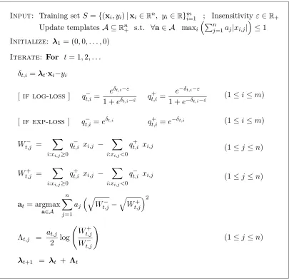
Figure 3: A log-additive update algorithm for minimizing either the log-loss or the exp-loss.
by setting the templates accordingly, and allows us to discuss and prove the correctness of both paradigms in a unified manner.
In this unified approach, we are required to pre-specify to the algorithm which subsets of
the coordinates ofλmay be updated simultaneously. Formally, the algorithm is given a set
of update templates A, where every templatea∈ Ais a vector in Rn
+. On every iteration,
the algorithm selects a template a∈ Aand updates only those elementsλj for which aj is
non-zero. We require that everya∈ Aconform with the constraintP
jaj|xi,j| ≤1 for all of
the instancesxi in the training set. The purpose of this requirement will become apparent
in the proof of Theorem 1. The parallel update is obtained by setting A to contain the
single vector (ρ, . . . , ρ) where ρ = (maxikxik1)−1. The sequential update is obtained by
setting Ato be the set of vectorsa1, . . . ,an defined by
ak,j=
(maxi|xi,j|)−1 ifj=k
The algorithm that we discuss is outlined in Figure 3 and operates as follows: during
the process of buildingλ, we may encounter two different types of discrepancies:
underes-timation and overesunderes-timation. If the predicted target λ·xi is less than the correct target
yi, we say that λ underestimates yi and if it is greater we say that λ overestimates yi.
For every instance-target pair in the training set, we use a pair of weights qt,i− and q+t,i to
represent its discrepancies: q−t,i represents the degree to whichyi is overestimated byλtand
analogouslyqt,i+ represents the degree to whichyiis underestimated byλt. We then proceed
to calculate two weighted sums over each coordinate of the instances: Wt,j− can be thought
of as the degree to whichλt,j should be decreased in order to compensate for overestimation
discrepancies. Symmetrically,Wt,j+ represents the degree to whichλt,j should be increased.
At this point, the algorithm selects the update template at ∈ A with respect to which it
will apply the update toλ. at is selected so as to maximize the decrease in loss, according
to a criterion that follows directly from Theorem 1 below. In the sequential version of the algorithm, selecting an update template is equivalent to selecting a single base regressor and updating its weight. In this case, the template selection criterion should be viewed as the
weak learning criterion of the boosting procedure. The algorithm’s iteration concludes with
an update of λ. Each element λj is updated by half the log ratio between the respective
elements of Wt+ and Wt−, times the scaling factorat,j.
The following theorem states a non-negative lower bound on the decrease in loss on every iteration of the algorithm for the case of the log-loss.
Theorem 1 Let {(xi, yi)}mi=1 be a training set of instance-target pairs where for all i in
1, . . . , m, xi∈Rn and yi∈R. Then using the notation defined in the algorithm outlined in
Figure 3, on every iteration tthe decrease in the log-loss satisfies,
Loss(λt, S) − Loss(λt+1, S) ≥
n
X
j=1 at,j
q
Wt,j− −
q
Wt,j+ 2
.
Proof Define ∆t(i) to be the difference between the loss attained by λtand that attained
by λt+1 on an instance-target pair (xi, yi) in the training set, namely
∆t(i) = Llog(δt,i)−Llog(δt+1,i). (4)
Since λt+1 = λt+Λt then δt+1,i = δt,i +Λt·xi. Using this equality, and the identity
1/(1 +eα) = 1−1/(1 +e−α), ∆
t(i) can be rewritten as
∆t(i) = −log
1 +eδt+1,i−ε
1 +eδt,i−ε
−log
1 +e−δt+1,i−ε
1 +e−δt,i−ε
= −log
1− 1
1 +e−(δt,i−ε) +
eΛt·xi 1 +e−(δt,i−ε)
−log
1− 1
1 +e−(−δt,i−ε) +
e−Λt·xi 1 +e−(−δt,i−ε)
.
We can now plug the definitions of qt,i+ andq−t,i into this expression to get
∆t(i) = −log
1−qt,i− 1−eΛt·xi
−log1−q+t,i 1−e−Λt·xi
Next we apply the inequality−log(1−α)≥α(which holds wherever log(1−α) is defined):
∆t(i) ≥ qt,i− 1−eΛt·xi + q+t,i 1−e−Λt·xi. (5)
We rewrite the scalar product Λt·xi in a more convenient form,
Λt·xi = n X j=1 at,j 2 log
Wt,j+/Wt,j−xi,j
=
n
X
j=1
(at,j|xi,j|) sign(xi,j) log
q
Wt,j+/Wt,j−. (6)
Recall the assumptions made on the vectors in A, namely that at and xi comply with
Pn
j=1at,j|xi,j| ≤1 and thatat,j|xi,j|is non-negative. This assumption is used in conjunction
with the fact that (1−eα) is a concave function and is equal to zero at α = 0. We can
replaceΛt·xi in Eq. (5) with the form given in Eq. (6) and use Jensen’s inequality to get,
∆t(i) ≥ qt,i− 1−e
Λt·xi
+qt,i+ 1−e−Λt·xi
≥
n
X
j=1
at,jqt,i−|xi,j|
1−esign(xi,j) log
“q
Wt,j+/W−
t,j ” + n X j=1
at,jqt,i+|xi,j|
1−e−sign(xi,j) log
“q
Wt,j+/Wt,j−” .
We now rewrite,
∆t(i) ≥
X
j:xi,j>0
at,jq−t,i|xi,j|
1− v u u t
Wt,j+ Wt,j−
+ X
j:xi,j<0
at,jq−t,i|xi,j|
1− v u u t
Wt,j− Wt,j+
+ X
j:xi,j>0
at,jq+t,i|xi,j|
1− v u u t
Wt,j− Wt,j+
+ X
j:xi,j<0
at,jq+t,i|xi,j|
1− v u u t
Wt,j+ Wt,j−
.
Summing ∆t(i) over iand using the definition of theq’s andW’s we finally get that,
m
X
i=1
∆t(i) ≥
n
X
j=1 at,j
Wt,j−1−
q
Wt,j+/Wt,j−+Wt,j+ 1−
q
Wt,j−/Wt,j+
= n X j=1 at,j q
Wt,j− −
q
Wt,j+ 2
.
This concludes the proof.
Theorem 1 focuses on the log-loss function, but is easily adapted to case of the exp-loss. Note that the only difference between the log-loss and exp-loss cases in the algorithm
pseudo-code (Figure 3) is in the definitions of the overestimation and underestimation weightsq−
and q+. When our goal is to minimize the exp-loss, we define
qt,i− = eδt,i q+
To show that Theorem 1 still holds for the exp-loss we modify the definition of ∆t(i) from
Eq. (4) in accordance to the change in the loss. Specifically, let
∆t(i) = Lexp(δt,i)−Lexp(δt+1,i)
= eδt,i−eδt+1,i+e−δt,i−e−δt+1,i.
As before, we plug the definitions ofqt,i+ and qt,i− from Eq. (7) into the above and rewrite ∆t
as,
∆t(i) = q−t,i 1−eΛt·xi+q+t,i 1−e−Λt·xi.
Eq. (5) in the proof of Theorem 1 now holds with equality and the rest of the proof proceeds as before. Consequently, we get the same lower bound for the exp-loss as was stated in Theorem 1 for the log-loss.
Similarly, we can redefine q− and q+ to minimize the loss. Recall that the
comb-loss function is defined by a pair of insensitivity parameters, ε1 and ε2. To minimize the
comb-loss, we define
qt,i− = e
δt,i−ε1
1 +eδt,i−ε1 + e
δt,i−ε2 q+ t,i =
e−δt,i−ε1
1 +e−δt,i−ε1 + e
−δt,i−ε2.
Again, the formal discussion given in this section carries over to the comb-loss case with only minor technical adaptations necessary.
To conclude this section, we note that the log-additive algorithm can be used verbatim in
the case of aweightedloss. In Section 4 we use this extension to devise a simple regularization
scheme. Formally, letν ∈Rm
+ be a vector of non-negative weights such thatνi is the weight
of the i’th example. The weighted loss is defined as,
Loss(λ,ν, S) =
m
X
i=1
νiL(λ·xi−yi),
where L(·) is any of the loss functions discussed above. The sole change to the algorithm
resides in the calculation of the weightsq+t,iandqt,i− which must now be scaled byνi, namely,
qt,i+ ←νiqt,i+ andq−t,i ←νiq−t,i. It is easy to verify that Theorem 1 still holds for this extended
definition of weighted-loss.
3. Additive Update for Batch Regression
In this section we describe a family of additive batch learning algorithms that advance on each iteration in a direction which is a linear transformation of the gradient of the loss. We
term these algorithmsadditive update algorithms. These algorithms bear a resemblance to
the log-additive algorithms described in the previous section, as do their proofs of progress. As in the previous section, we first restrict the discussion to the log-loss and then outline the adaptation to the exp-loss at the end of the section.
We again devise a template-based family of updates. This family includes a parallel
update which modifies all the elements ofλ simultaneously and a sequential update which
updates a single element ofλon each iteration. The parallel update amounts to a gradient
Input: Training set S={(xi, yi)|xi ∈Rn, yi ∈R}mi=1 ; Insensitivityε∈R+
Update templates A ⊆Rn
+ s.t. ∀a∈ A
Pm
i=1
Pn
j=1ajx2i,j ≤2
Initialize: λ1 = (0,0, . . . ,0)
Iterate: For t= 1,2, . . .
δt,i=λt·xi−yi
[ if log-loss ] qt,i− = e
δt,i−ε
1 +eδt,i−ε q
+ t,i =
e−δt,i−ε
1 +e−δt,i−ε (1≤i≤m)
[ if exp-loss ] qt,i− = e
δt,i
Zt
q+t,i = e−
δt,i
Zt
(1≤i≤m)
where Zt=
m
X
i=1
eδt,i+e−δt,i+ 2
Wt,j = m
X
i=1
(qt,i+ −q−t,i)xi,j (1≤j≤n)
at= argmax
a∈A
n
X
j=1 ajWt,j2
Λt,j = at,jWt,j (1≤j≤n)
λt+1 = λt + Λt
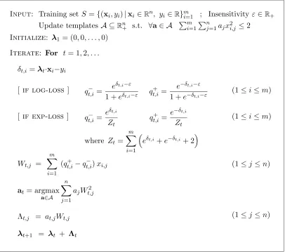
Figure 4: An additive update algorithm for minimizing either the log-loss or the exp-loss.
λj is an axis-parallel gradient descent step. We denote the set of update templates by
A and assume that every a ∈ A is a vector in Rn
+. For each a ∈ A we require that
Pm
i=1
Pn
j=1ajx2i,j ≤2.
The pseudo-code of the additive update algorithm is given in Figure 4. Intuitively, on
each iteration t, the algorithm computes the negative of the gradient with respect to λt,
denoted (Wt,1, . . . , Wt,n). It then selects the update template at∈ A which, as we shortly
show in Theorem 2, guarantees a maximal drop in the loss. Finally, λt,j is updated by
at,jWt,j.
Theorem 2 Let {(xi, yi)}mi=1 be a training set of instance-target pairs where for all i in
1, . . . , m, xi∈Rn and yi∈R. Then using the notation defined in the algorithm outlined in
Figure 4, on every iteration tthe decrease in the log-loss, denoted ∆t, satisfies
∆t = Loss(λt, S) − Loss(λt+1, S) ≥ 1
2
n
X
j=1
Proof We begin by defining a quadratic function Q:R→R which is parameterized by
two parameters,λ and Λ. Qλ,Λ will be shown to be an upper bound on the log-loss along
the directionΛ from λ. Concretely,Qλ,Λ is defined as,
Qλ,Λ(α) = Loss(λ, S) + (∇Loss(λ, S)·Λ) α−α2/2
.
Formally, we show that for all α, Qλt,Λt(α)≥Loss(λt+αΛt, S) whereΛt is defined as in
Figure 4. For convenience, we define Γ(α) = Qλt,Λt(α)−Loss(λt+αΛt, S) and instead
prove that Γ is a non-negative function.
By construction, we get that Γ(0) = 0. Since the derivative of Qλt,Λt at zero is equal
to ∇Loss(λt, S)·Λt, we get that the derivative of Γ at zero is also zero. To prove that Γ
is a non-negative function it remains to show that Γ is convex and thus α = 0 attains its
global minimum. To prove convexity it is sufficient to show that the second derivative of Γ
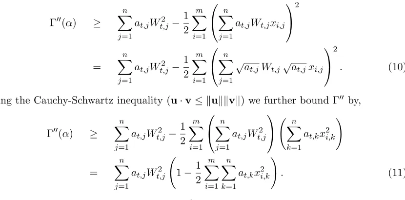
(denoted Γ00) is non-negative. Routine calculations yield that,
Γ00(α) = −Λ· ∇Loss(λ, S)−ΛTHΛ, (8)
whereH =Pm
i=1L 00
log(λ+αΛ)xix T i andL
00
logis the second derivative of the log-loss function.
It is simple to show that this derivative is bounded in [0,1/2]. Plugging the value ofH into
Eq. (8) we get that,
Γ00(α) ≥ −Λ· ∇Loss(λ, S)−1
2
m
X
i=1
(Λ·xi)2. (9)
Note that on the t’th iteration, the j’th element of Λt equals at,jWt,j where Wt,j =
−∇jLoss(λt, S). Therefore, we rewrite Eq. (9) as,
Γ00(α) ≥
n
X
j=1
at,jWt,j2 −
1 2 m X i=1 n X j=1
at,jWt,jxi,j
2 = n X j=1
at,jWt,j2 −
1 2 m X i=1 n X j=1 √a
t,jWt,j√at,jxi,j
2
. (10)
Using the Cauchy-Schwartz inequality (u·v≤ kukkvk) we further bound Γ00 by,
Γ00(α) ≥
n
X
j=1
at,jWt,j2 −
1 2 m X i=1 n X j=1
at,jWt,j2
n
X
k=1
at,kx2i,k
!
=
n
X
j=1
at,jWt,j2 1−
1 2 m X i=1 n X k=1
at,kx2i,k
!
. (11)
Finally, we use the constraintP
i
Pn
k=1at,kx2i,k ≤2 which immediately implies that Γ00(α)≥
0. Summing up, we have shown that Loss(λt+αΛt, S) is upper bounded by Qλt,Λt(α).
Therefore, Loss(λt+1, S) = Loss(λt+Λt, S) ≤ Qλt,Λt(1), hence,
∆t ≥ Loss(λt, S) − Qλt,Λt(1) =
1 2
n
X
j=1
This concludes the proof.
To conclude this section, we briefly outline the adaptation of the additive update algo-rithm to the exp-loss. Recall that in the exp-loss setting, our goal is to minimize,
m
X
i=1
eδi+e−δi
where δi =λ·xi−yi.
Since the gradient of the exp-loss is itself exponential, we cannot hope to minimize the exp-loss by straightforward gradient descent. However, instead of minimizing the exp-loss function over the sample, we can minimize the loss,
log
m
X
i=1
eδi+e−δi+ 2 !
. (12)
Clearly, both functions attain the same (global) minimum. We can now repeat verbatim the
proof technique of Theorem 2 usingq− and q+as defined for the exp-loss case in Figure 4.
The additive update family of algorithms can accommodate a weighted loss just as log-additive update algorithms do. The algorithm is adapted to cope with weights in the same way that the log-additive algorithm was adapted in the end of Section 2, namely by an
appropriate rescaling of the weights q− and q+.
4. Regularization
Regularization is a means of controlling the complexity of the regressor being learned. In particular for linear regressors, regularization serves as a soft limit on the magnitude of the
elements of λ(cf. (Poggio and Girosi, 1990)). The loss functions discussed in the previous
sections can also be used as a new form of regularization. Using the log-loss, we can apply
the following regularization to thej’th coordinate ofλ,
log1 +eλj
+ log1 +e−λj
.
The minimum of the above equation is obtained at λj = 0. It is straightforward to show
that the regularization term above is bounded from below by|λj|and from above by|λj|+2.
Therefore, summing over all possible indices j, the regularization term on λ lies between
kλk1 and kλk1+ 2n. Thus, this form of regularization can be viewed as a smooth
approx-imation to the `1 norm of λ. A similar form of regularization can be imposed using the
exp-loss, namely,
eλj+e−λj.
For both losses, the j’th regularization term equals L(λj; 0). When the set of base
hy-potheses is finite, an equivalent way to impose this form of regularization is to introduce
a set of pseudo examples Sreg = {xk,0}nk=1 where xk = 1k (the vector with 1 in its k’th
position and zeros elsewhere). Let ν > 0 be a regularization parameter that governs the
relative importance of the regularization term with respect to the empirical loss. Slightly
overloading our notation, let Loss(λ, ν, S) denote the regularized empirical loss, defined by,
As noted in Section 2 and Section 3, both the log-additive and additive update batch
algorithms easily accommodate a weighted loss. Therefore, by introducing a set ofn
pseudo-examples, each of which weighted by ν, we can incorporate regularization into our batch
algorithms without any modification to the algorithm core. Concretely, we set the weight
of each example inS to 1 and of each pseudo-example inSreg toν. We can now use either
the log-additive or the additive algorithm to minimize the weighted loss.
In practice, we do not need to explicitly add pseudo-examples to our sample in order to incorporate a regularization term into the loss function. A more efficient way of achieving the same effect is to modify our algorithms to behave as if such a pseudo sample was presented to them. For instance, for the log-additive log-loss update (Figure 3) the term
ν/(1 +e−λt,j) should be added to the definition ofW−
t,j for every coordinate being updated.
Analogously, the termν/(1 +eλt,j) should be added toW+
t,j. Applying this modification is
equivalent to adding pseudo-examples which correspond to the coordinates being updated.
Another useful property of this regularized loss is that it is strictly convex. To see
that Loss(λ, ν, S) is strictly convex it suffices to show that its Hessian is positive definite.
The Hessian of Loss(λ, ν, S) can be written as a sum of two matrices H+Hreg where the
first is the matrix of second order derivatives of Loss(λ, S) and the second contains the
second order derivatives ofνLoss(λ, Sreg). Since Loss(λ, S) is the sum of convex losses,H
is positive semi-definite. It is simple to verify that the matrix Hreg is a diagonal matrix
withHi,i = 2ν/ 1 +e−λi
1 +eλifor the log-loss orH
i,i=ν e−λi+eλi
for the exp-loss.
Clearly, the diagonal elements are strictly positive for both losses for any finiteλ. Therefore,
Hreg is positive definite and thus H+Hreg is positive definite as well. Furthermore, since
the regularization term tends to infinity at least as fast askλk1, the regularized loss has an
attainable global minimum. In other words, this form of regularization enforces uniqueness
of the solution in our loss minimization problem. We denote the unique global minimum of
Loss(λ, ν, S) byλ?. We use the uniqueness ofλ? in the next section where the convergence
of our batch algorithms is discussed.
5. Convergence
In the previous section we have argued that the regularized loss attains a unique minimum
at the point denotedλ?. In this section we show that the batch algorithms described so far
converge to this unique minimizer. For simplicity, we assume that the set of templates A
spans Rn. The following theorem can be tediously generalized to the case where the space
spanned byAis any linear-subspace ofRn in which case convergence is to the optimal value
within this subspace.
Theorem 3 Assume that the vectors in A span the entire space Rn. Let λ
1,λ2, . . . ,λt, . . .
be the sequence of vectors generated by the log-additive (Figure 3) or the additive (Figure 4) updates, using either of the regularized loss functions discussed in this paper. Then this
sequence converges to λ?, the global minimizer of the regularized loss L(λ, ν, S).
Proof Due to the introduction of the regularization term, the loss function is strictly convex
and attains its unique minimum at the point denotedλ?, as argued in the previous section.
within a compact set C. To see this, note that λ is initialized to be the zero vector and therefore the initial regularized loss is
Loss(0, ν, S) = Loss(0, S) + νLoss(0, Sreg).
Denote the initial loss above by L0. Since the loss attained by the algorithm on every
iteration is non-increasing, the contribution of the regularization term to the total loss
certainly does not exceedL0/ν. Also, the regularization term for both the exp-loss and the
log-loss bounds the `∞ norm of λtby
kλtk∞ ≤ Loss(λt, Sreg) ≤ Loss(λt, ν, S)/ν ≤ L0/ν.
Therefore, we can defineC ={λ:kλk∞≤ L0/ν}and assert that the sequenceλ1,λ2, . . .is
contained inC. Next, note that the lower bound on the decrease in loss given in Theorem 1
and Theorem 2 can be thought of as a function of the current regressor λt and the chosen
templateat. If the bound on the decrease equals zero for all possiblea∈ Athenλtmust be
equal toλ?. Otherwise, there existsa∈ Afor which the decrease bound is strictly positive.
To see this, note that if the decrease bound for the log-additive update is 0 then,
∀j: qWt,j− −
q
Wt,j+ 2
= 0,
which implies that Wt,j− −Wt,j+ = 0. Note that Wt,j− −Wt,j+ is the j’th partial derivative of the loss function being minimized (log-loss, exp-loss, or comb-loss). Since the regularized loss function is strictly convex, a zero gradient vector is attained only at the optimal point
λ?. A similar argument holds for the additive update.
Assume now by contradiction that the sequence of regressors λ1,λ2, . . . does not
con-verge toλ?. An immediate consequence of this assumption is that there exists γ >0 such
that an infinite subsequence of regressorsλs1,λs2, . . .remains outside ofB(λ
?, γ), the open
ball of radius γ centered at λ?. The set C \B(λ?, γ) is a compact set and therefore the
lower bound from Theorem 1 (or equivalently Theorem 2) attains a minimum value over
C\B(λ?, γ) at some point ˜λ. Denote this minimum byµ. Since ˜λ6∈B(λ?, γ) it necessarily
follows that ˜λ6=λ?and thereforeµmust be strictly positive. Thus, on each of the iterations
s1, s2, . . . the decrease in loss is at least µ > 0. The subsequence s1, s2, . . . is infinite and
as a consequence the loss must eventually become negative. We get a contradiction since
the loss is a non-negative function. We conclude that the sequenceλtmust converge toλ?.
6. Back to Classification
To conclude the part of the paper which discusses batch algorithms we would like to briefly draw connections to boosting algorithms for classification. The reader mainly interested in regression problems may skip this section.
setting we receive a training setS ={(x1, y1), . . . ,(xm, ym)} where each target yi is either
−1 or +1. As in the case of regression,xis the mapping of an instance into its image under
the set of base-classifiers, x 7→ (h1(x), . . . , hn(x)) and the goal is to find a function f(x)
that attains a small loss. The functionf(x) is a weighted combination of base-hypotheses,
f(x) = Pn
j=1λjhj(x) = λ·x. The skeleton of the additive algorithm for classification
is almost the same as the one for regression. In the classification case we define a single
(unnormalized) distribution over the examples, setting the weight of the i’th example to,
qt,i=e−δt,i/Zt [exp-loss ] ; qt,i=
1
1 +e−δt,i [log-loss ],
where δi =yiλt·xi and Zt= 1 +Pmi=1e−δt,i. On roundt we set each variable Wt,j to be
Wt,j =Pni=1qt,ixi,j. The rest of the algorithm, including the constraint Pi,jajx2i,j ≤2, is
kept intact. The result is a new boosting-type procedure where base-hypotheses are selected
so as to maximizeP
jajWi,j2 .
The regularization technique discussed in Section 4 can be used in classification tasks as well. It is worth noting that Schapire et al. (2002) suggested a procedure for incorporating prior knowledge into log-loss boosting which can also be used for regularization. We compare the two regularization techniques in the log-loss case. Using the notation of Section 4, the regularization technique of Schapire et al. can also be described via the introduction of a
pseudo-sample. Given a training set S={xi, yi}i=1m withyi ∈ {−1,+1} define the
pseudo-sample ¯S ={xi,−yi}and use log-loss boosting to train a classifier whose task is to minimize
the loss,
(1−ν)Loss(λ, S) +νLoss(λ,S¯),
where, as before,ν is a regularization parameter. In this caseν is restricted to the interval
[0,1/2]. This construction of a regularization sample implies that even when there exists a
strong-hypothesis which attains zero classification error onS the extended sampleS∪S¯ is
inseparable. If the space spanned by the examples is of a full rank, then this regularization
scheme guarantees a unique and attainable global minimizerλ?. However, the two optima
due to the two different regularization schemes will be achieved at different points. The
regularization scheme presented in this paper penalizes large values of|λj|whereas Schapire
et al. penalize overconfident predictions.
7. Online Regression Algorithms
In this section we describe online regression algorithms for the log-loss defined in Eq. (1).
In the previous sections we allowed ourselves to ignore the constant κ which appears in
the definition of the log-loss since this did not alter the global minimum of our problem.
However, in the online learning setting this constant should not be ignored. Inclusion of κ
does not affect the online algorithms themselves as they depend only on the gradient of the loss function, but it will play a role in their analysis.
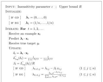
We follow the notation and techniques presented in (Kivinen and Warmuth, 1997; Cesa-Bianchi, 1999). In online learning settings, we observe a sequence of instance-target pairs,
in rounds, one by one. On round t we first receive an instance xt. Based on the current
regressor,λt, we extend a prediction λt·xt. We then receive the true target yt and suffer
Input: Insensitivity parameterε ; Upper boundR
Initialize:
[ if gd ] λ1 = (0, . . . ,0)
[ if eg ] λ1= (1/n, . . . ,1/n)
Iterate: For t= 1,2, . . .
Receive an examplext
Predict λt·xt
Receive true targetyt
Update:
δt=λt·xt
Llog0 (δt) = 1+e−1δt+ε − 1+e1δt+ε
βt=L 0
log(δt)/R
[ if gd] λt+1,j=λt,j−βtxt,j (1≤j≤n)
[ if eg] λt+1,j= λt,je −βt xt,j
Pn k=1λt,ke
−βt xt,k (1≤j≤n)
Figure 5: The GD and EG algorithms for online regression with the log-loss.
The learning algorithm employs an update rule which modifies its current regressor after each round. We describe and analyze two online regression algorithms for the log-loss that differ in the update rules that they employ. The first is additive in the gradient of the loss
and is thus called Gradient Descent (GD) while the second is exponential in the gradient
of the loss and is analogously calledExponentiated Gradient (EG).
The GD algorithm: The pseudo-code of the algorithm is given in Figure 5. Note that
the GD algorithm updates its current regressor, λt, by subtracting the gradient of the loss
function from it. The GD algorithm assumes an upper boundRon twice the squared norm
of all the instances, that is, 2kxtk22 ≤R. In the following analysis we give a bound on the
cumulative loss attained on any number of rounds. However, rather than bounding the
loss per se we bound the cumulative loss relativeto the cumulative loss suffered by a fixed
regressor µ. The bound holds for any linear regressor µand any number of rounds, hence
we get that the GD algorithm is competitive with the optimal (fixed) linear regressor for any number of rounds. Formally, the following theorem states that the cumulative loss attained by the GD algorithm is at most twice the cumulative loss of any fixed linear regressor plus an additive constant.
Theorem 4 Let S ={(x1, y1), ...,(xT, yT)}be a sequence of instance-target pairs such that
(Figure 5) on the sequence. Then for any fixed linear regressor µ∈Rn we have
T
X
t=1
Llog(λt·xt−yt) ≤ 2
T
X
t=1
Llog(µ·xt−yt) + Rkµk22 . (13)
Note that the statement of the theorem changes if the constant κ is excluded from the
definition of the log-loss in Eq. (1), resulting in a looser bound. The proof of the theorem is based on the following lemma that underscores an invariant property of the update rule.
Lemma 5 Consider the setting of Theorem 4, then for each round t we have
Llog(λt·xt−yt)−2Llog(µ·xt−yt) ≤ R kλt−µk22− kλt+1−µk22
. (14)
The proof of the lemma is given in Appendix A. Intuitively, the lemma states that if the loss
attained byλt on roundtis greater than the loss of a fixed regressorµ, then the algorithm
will update λtsuch that it gets closer to µ. In contrast, if the loss of µis greater than the
loss of GD, the algorithm may move its regressor away fromµ. With Lemma 5 handy, the
proof of Theorem 4 is almost immediate.
Proof of Theorem 4: Summing Eq. (14) fort= 1, ..., T we get
T
X
t=1
Llog(λt·xt−yt)−2 T
X
t=1
Llog(µ·xt−yt) ≤ R kλ1−µk22− kλT+1−µk22
≤ Rkλ1−µk22
= Rkµk22,
where in the last equality we use the fact that the initial regressor,λ1, is the zero vector.
The EG algorithm: The algorithm is described in Figure 5 and works under the
as-sumption that the regressorλis contained in the probability simplex, namelyλ∈Pnwhere
Pn = {µ : µ ∈ Rn +,
Pn
j=1µj = 1}. We note in passing that following a construction
described in (Kivinen and Warmuth, 1997), it is possible to derive a generalized version
of EG in which the elements of λ can be either negative or positive, so long as the sum
of their absolute values is less than 1. The EG algorithm assumes an upper bound on the squared difference between the maximal and minimal coordinates of the instances it
receives, R≥(maxjxt,j −minjxt,j)2. Since EG maintains a regressor from the probability
simplex, we measure the cumulative loss of the EG algorithmrelativeto the cumulative loss
achieved by any fixed regressor from the probability simplex.
Theorem 6 Let S ={(x1, y1), ...,(xT, yT)}be a sequence of instance-target pairs such that
∀t : (maxjxt,j −minjxt,j)2 ≤ R and let λ1, ...,λT be the regressors generated by the EG
online algorithm (Figure 5) on the sequence. Then, for any fixed regressor µ∈Pn we have
T
X
t=1
Llog(λt·xt−yt) ≤
4 3
T
X
t=1
Llog(µ·xt−yt) +
4R
3 DRE(µ,λ1) , (15)
where DRE(p, q) =
P
The proof of the theorem is analogous to the proof of Theorem 4 and employs the following relative entropy based progress lemma.
Lemma 7 Consider the setting of Theorem 6, then for each round t we have
Llog(λt·xt−yt)−
4
3Llog(µ·xt−yt) ≤
4R
3 (DRE(µ,λt)−DRE(µ,λt+1)) . (16)
The proof of the lemma is given in Appendix A.
8. Experiments
In this section we present experimental results that demonstrate different aspects of our algorithms in the light of their formal analysis. In Section 8.1, we start with a synthetic example that underscores the different properties of the log-loss and the exp-loss functions. We then turn to a comparison of the different algorithmic approaches to minimizing these losses. In Section 8.2 we compare the log-additive and additive batch updates by examining how certain properties of the training data influence the rates of convergence of the two updates. Next we demonstrate the different benefits of the sequential and parallel update paradigms. In Section 8.3 we use the sequential form of our update as a boosting procedure which uses regression stumps as base regressors. We compare this boosting technique to the LAD algorithm (Friedman, 2001) on a natural data set. In Section 8.4 we turn our attention to the parallel update paradigm. When using the parallel update, some form of regularization is essential to avoid over-fitting. We therefore demonstrate the effectiveness of the regularization scheme presented in Section 4 and show the effect of the regulariza-tion parameter on the generalizaregulariza-tion ability of our algorithms. More specifically, we learn a kernel-based regressor and compare our log-loss regularization to Support Vector Regression
with l1 regularization. The last two experiments illustrate some properties of our online
algorithms and are presented in Section 8.5. In these experiments, we compare the cumu-lative loss of the online GD algorithm with its theoretical bound given in Theorem 4. We also compare the sensitivity of the online GD and EG regression algorithms to the number of relevant coordinates in the data, demonstrating that EG vastly outperforms GD when the number of relevant coordinates is small.
8.1 Comparison of the Exp-Loss and the Log-Loss
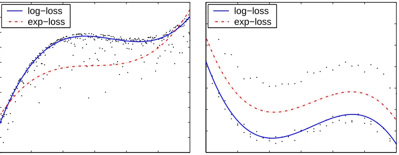
In this section we describe an experiment that underscores the different merits of the log-loss and the exp-log-loss functions. The end result is that the solution obtained by minimizing
the log-loss shares the same asymptotic behavior as the `1 regression loss (Pi|δi|). On
the other hand, the solution found by minimizing the exp-loss approximately minimizes
the l∞ regression loss on the sample. To exemplify the above properties we created two
synthetic data sets and for each one we found the two regressors that minimize the log-loss and the exp-loss respectively. The two data sets and the resulting regressors are depicted in Figure 6. Each of the two data sets was generated by sampling points on the curve of
a univariate third degree polynomial, resulting in a sampleS ={(xi, yi)} wherexi, yi ∈R.
log−loss exp−loss
log−loss exp−loss
Figure 6: A comparison of log-loss and exp-loss on synthetic data.
normally with a zero mean and a variance of 0.1. In the first experiment, the targets were
further contaminated by adding one-sided noise which was generated by subtracting the absolute value of a normal variable with a zero mean and a unit variance (Figure 6, left).
Each instance xi was expanded by taking powers of xi, i.e. we performed the mapping
xi 7→ (1, xi, x2i, x3i). This expansion enables us to use our linear algorithms to learn degree
three polynomials. It is clear from the figure that the regressor obtained by minimizing the log-loss is very close to the polynomial generating the data, demonstrating the robustness of the log-loss to biased noise. The regressor attained by minimizing the exp-loss, however, approximately minimizes the maximal discrepancy over the entire data set and therefore lies significantly below. The other facet of this behavior is illustrated on the right hand side
of Figure 6. In this data set, the additional one sided noise was set toonewith a probability
of 1/3 and otherwise it was set to zero. Thus, about a third of the targets were shifted up
by 1. Here, the regressor obtained by minimizing the exp-loss lies between the two groups
of points and as such approximately minimizes the `∞ regression loss on the sample. The
regressor found by minimizing the log-loss practically ignores the samples that were shifted
by 1 and as such approximately minimizes the `1 regression loss on the sample.
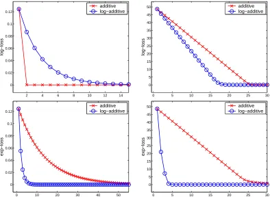
8.2 A Comparison of the Log-Additive and Additive Updates
In this section we compare the performance of the log-additive update from Figure 3 to that of the additive update from Figure 4. An important difference between the two updates is the type of constraint imposed on the norm of the update templates. In the following, we demonstrate the effect of this difference on the convergence rates of the two update strategies. To make the comparison as simple as possible, we chose the instance space to
beR1. Therefore, the instances are scalars and there is a single update templatea∈R. For
the log-additive update the constraint on abecomes amaxi|xi| ≤1 while for the additive
update the constraint isaP
ix2i ≤2. To demonstrate the implications of the different norm
constraints, we generated two synthetic data sets. The target of each instance was set for
both data sets to be equal to the input instance, that is, yi =xi. Each data set consists
of 26 instance-target pairs. For both data sets, we set the value of the first 25 instances to
2 4 6 8 10 12 14 0
0.02 0.04 0.06 0.08 0.1 0.12
log−loss
additive log−additive
0 5 10 15 20 25 30
0 5 10 15 20 25 30 35 40 45 50
log−loss
additive log−additive
0 10 20 30 40 50
0 0.02 0.04 0.06 0.08 0.1 0.12
exp−loss
additive log−additive
0 5 10 15 20 25 30
0 5 10 15 20 25 30 35 40 45 50
exp−loss
additive log−additive
Figure 7: Comparison of the convergence rates of the log-additive and additive updates on two different data sets (see text). The left column corresponds to the first data set and the right column to the second. The top row presents results for the log-loss while the bottom row presents results for the exp-loss.
we set it to 10. Therefore, for the first data set, the constraint onareduces to a≤2 when
using the log-additive update and to a≤4 when the additive update is used. In the case
of the second data set, the constraint on a becomesa ≤0.02 for the log-additive update,
and a≤0.0008 for the additive one. We would like to note in passing that for the additive
update, atypically decreases as the number of examples increases. Hence, the steps that
additive update takes are likely to be smaller in large data sets. The end result is slower convergence rates as both the log-additive and the additive updates scale linearly with the
value of the template used. Put another way, a small value of a yields an update which
changes λ rather conservatively. Therefore, in the settings discussed in this section, the
Another important difference between the two updates is the construction ofqi+andq−i
when minimizing the exp-loss. Recall that in the case of the log-additive update, the weights of the examples are qi+=eδi and q−
i =e−δi while for the additive update we further divide
these weights byZ. Therefore, when the data set contains examples for which the exp-loss
cannot be made small, the value of Z is likely to be rather large. Unlike the log-additive
update, the additive form issensitiveto scaling of the weightsqi+andqi−. Thus, wheneverZ
is large, the resulting normalized weights will be small and therefore the corresponding step sizes taken by the additive update will also be small. The bottom row of Figure 7 reflects this sensitivity of the additive update to scaling. For both data sets described above the log-additive update exhibits much faster convergence than the additive-one.
8.3 Boosting Regression Stumps
The next experiment demonstrates the effectiveness of the log-additive and additive updates in their sequential form, when they are applied as boosting procedures. As in the classic boosting setting, our algorithm has access to an external learning procedure called a base or weak learner. The goal of the boosting algorithm is to construct a highly accurate regressor by combining base regressors obtained from consecutive calls to the base learner. On every
boosting iteration the base learner receives the training set along with the weights qt,i+ and
qt,i− generated by the boosting algorithm. The goal of the base learner is to construct a
regressor which maximizes the decrease in loss. We denote by ht :Rn → R, the regressor
returned by the base learner on round t. We use either the bound in Theorem 1 or the
bound in Theorem 2 as the criterion for selecting a base regressor using the log-additive and additive updates respectively. That is, the base learner attempts to maximize the lower bound on the decrease in loss given in Theorem 1 or Theorem 2.
In our experiments, we use regression stumps as base regressors. Like decision stumps
which are depth-one decision trees, regression stumps are the simplest form of regression trees (cf. Friedman (2001)). Each stump is characterized by two parameters: a feature index
parameter, `∈ {1, . . . , n} and a threshold parameter θ∈R. The prediction of each stump
is either−1 or +1 and is defined ash(x) = sign(θ−x`). We now describe the specific base
learner we use. Given a training set S={(xi, yi)}of minstance-target pairs, we construct
for each feature index ` ∈ {1, . . . , n} a set of candidate thresholds. Each set consists of
all possible mid-points between two consecutive values of that feature on the training set.
Formally, let Θ` denote the candidate thresholds set for feature`and letxi,`denote the`th
feature of the ith instance inS. Then, the set Θ` is defined as,
Θ`={(xi1,`+xi2,`)/2|xi1,`< xi2,` and @r s.t. xi1,`< xr,` < xi2,`}. (17)
Note that each set Θ` may contain at most m −1 different thresholds and can be
pre-computed efficiently in time mlog(m) by sorting the training set independently for each
feature.
Given the current set of weights, q+t,i and q−t,i, the base learner constructs a regression
stump by choosing a feature index ` and a threshold value θ∈Θ`. This pair is chosen so
as to maximize the bound on the decrease in the log-loss as defined in Theorem 1 or in Theorem 2. It is easy to verify that the value of an update template for each base regressor
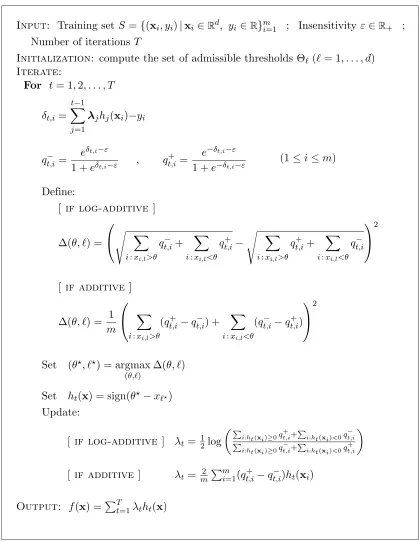
Input: Training setS ={(xi, yi)|xi ∈Rd, yi ∈R}mi=1 ; Insensitivityε∈R+ ;
Number of iterations T
Initialization: compute the set of admissible thresholds Θ`(`= 1, . . . , d)
Iterate:
For t= 1,2, . . . , T
δt,i = t−1
X
j=1
λjhj(xi)−yi
q−t,i = e
δt,i−ε
1 +eδt,i−ε , q
+ t,i=
e−δt,i−ε
1 +e−δt,i−ε (1≤i≤m)
Define:
[ if log-additive ]
∆(θ, `) =
s
X
i:xi,l>θ
q−t,i+ X
i:xi,l<θ
qt,i+ −
s X
i:xi,l>θ
q+t,i+ X
i:xi,l<θ
qt,i−
2
[ if additive ]
∆(θ, `) = 1
m
X
i:xi,l>θ
(q+t,i−qt,i−) + X
i:xi,l<θ
(qt,i− −qt,i+)
2
Set (θ?, `?) = argmax
(θ,`)
∆(θ, `)
Set ht(x) = sign(θ?−x`?)
Update:
[ if log-additive] λt= 12log
P
i:ht(xi)≥0q
+
t,i+
P
i:ht(xi)<0q−t,i
P
i:ht(xi)≥0q
−
t,i+
P
i:ht(xi)<0q
+
t,i
[ if additive ] λt= m2 Pmi=1(qt,i+ −q−t,i)ht(xi)
Output: f(x) =PT
t=1λtht(x)
since the output of the base regressors is either +1 or−1. Hence, given a candidate feature
index`and a thresholdθ∈Θ` the bound on the decrease in loss for the additive update is,
1
m
X
i:xi,l>θ
(qt,i+ −q−t,i) + X
i:xi,l<θ
(qt,i− −qt,i+)
2
, (18)
and for the log-additive update the bound is,
s
X
i:xi,l>θ
qt,i− + X
i:xi,l<θ
q+t,i−
s X
i:xi,l>θ
qt,i+ + X
i:xi,l<θ
q−t,i
2
. (19)
As mentioned above, the base learner evaluates one of the above terms (depending on the
update) for each possible ` and θ ∈ Θ`. It then chooses the pair which maximizes either
Eq. (18) or Eq. (19). The pseudocode of the regression learning algorithm using stumps for both the additive and the log-additive updates is given in Figure 8.
We compared the regression algorithm with stumps to an algorithm named Least Ab-solute Deviation (LAD) due to Friedman (2001). LAD is a boosting-style algorithm which attempts to minimize the hinge-loss by fitting a base hypothesis to the residual error, the approximation error left after applying the combination of base hypotheses found so far. It is not obvious how to conduct a fair comparison between our approach and LAD since the direct objective of our regression learning algorithm is to minimize the log-loss while the goal of LAD is to minimize the hinge-loss. To remove any doubt on the validity of the results, we evaluate both algorithms using the hinge-loss, thus giving a slight advantage to LAD in our empirical evaluation. In addition, we compared the mean squared errors (MSE) of the algorithms.
We ran experiments on two standard data sets for regression: the Boston housing data
set from the UCI repository and thebody fat data set (Penrose et al., 1985). To evaluate our
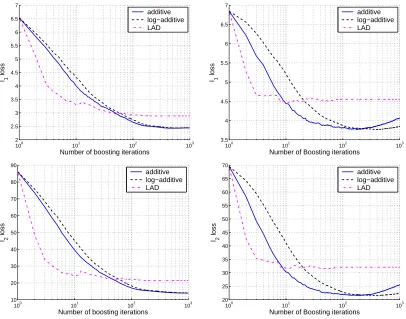
results, we used a 10-fold cross validation technique. The plots on the top row of Figure 9 depict the average hinge-loss on the two data sets as a function of the number of sequential iterations while the plots on the bottom row correspond to the mean squared error obtained by the algorithms on the same data sets. The plots underscore a few interesting phenomena. The LAD algorithm appears to be able to decrease the hinge loss and the MSE much faster than our algorithm on both the training data (not shown) and the test data. In no more than 3 iterations, LDA is able to achieve rather low loss. It takes about an order of magnitude more iterations for our algorithm to obtain the same performance LAD achieves after 2 or 3 iterations. This behavior can be partially attributed to the fact that LAD is designed to directly maximize the decrease in loss while our algorithm maximizes a lower bound on the decrease in loss. However, despite its initial performance, LDA seems to “get stuck” rather quickly and the final regressor it obtains has substantially higher loss on both data sets compared to our algorithm, whether it is trained with the log-additive update or the additive one. The improved generalization performance may be attributed to the following behavior that is common to boosting algorithms: as more base regressors are added, the
regression error obtained on most of the examples is rather small. Thus, the weights q+i
100 101 102 103 2
2.5 3 3.5 4 4.5 5 5.5 6 6.5 7
Number of boosting iterations
l1
loss
additive log−additive LAD
100 101 102 103
3.5 4 4.5 5 5.5 6 6.5 7
Number of Boosting iterations
l1
loss
additive log−additive LAD
100 101 102 103
10 20 30 40 50 60 70 80 90
Number of boosting iterations
l2
loss
additive log−additive LAD
100 101 102 103
20 25 30 35 40 45 50 55 60 65 70
Number of Boosting iterations
l2
loss
additive log−additive LAD
Figure 9: A comparison of the`1and MSE losses obtained by the regression algorithm with
stumps and the LAD algorithm (see text) on Boston housing data set (left) and body-fat (right) data sets.
decreases in the loss. Thus, even simple regressors such as decision stumps can further reduce the loss on the remaining examples for which the loss is still high. Indeed, we see that some over-fitting takes place when our regression algorithm is run for more than 200 iterations.
Comparing the performance of the additive and the log-additive updates in this exper-iment, it is apparent that the former seems more effective in reducing the loss but is also more susceptible to over-fitting. The accuracy of each update strategy seems to be prob-lem dependent. We leave further theoretical and empirical research on the generalization properties of the two updates to future research.
8.4 Examining the Effect of Regularization
10−10 10−5 100 105 0
2 4 6 8 10 12
l1
−loss
ν
train test
10−10 10−5 100 105
0 1 2 3 4 5 6 7
l1
−loss
ν
train test
Figure 10: The training and test losses as a function of the regularization parameter (ν) for
the log-loss (left) and Support Vector Regression (right).
regularization can ensure that the generalization loss (i.e. the regression loss suffered on test examples) would not greatly exceed the loss obtained on the training set. The feature space we use in this experiment is based on kernel operators. Concretely, the regressors we construct take the form
fλ(x) =
m
X
j=1
λjk(xj,x),
where{x1, . . . ,xm}are the instances in the training set andkis a kernel function. We used
the log-additive and additive update algorithms to minimize the following regularized loss,
Loss(λ, ν, S) =
m
X
i=1
Llog(fλ(xi)−yi;ε) + ν
m
X
j=1
Llog(λj). (20)
As illustrated in Figure 1, the log-loss can be interpreted as a smooth approximation to the
ε-insensitive hinge loss used by Support Vector Regression (SVR). SVR is a technique for
non-linear regression which uses kernel functions. For a thorough review of SVR, see for
instance (Smola and Sch¨olkopf, 1998). In our setting, the regularized loss from Eq. (20) can
be viewed as a smooth approximation to the hinge-loss with l1 regularization that is used
in Linear Programming Support Vector Regression (LP-SVR), namely,
m
X
i=1
|fλ(xi)−yi|ε + ν
m
X
j=1
|λj|. (21)
We ran experiments using theBoston Housing data set from the UCI Machine Learning
Repository. Following Bi and Bennett (2003), we chose to use a Gaussian kernel with
2σ2 = 3.9. We ran experiments with set to 0,1,2,3. The preprocessing we performed
consisted of shifting and scaling the input variables to the unit hypercube. Specifically, let
−12 −10 −8 −6 −4 −2 0 2 4 0
1 2 3 4 5 6 7 8 9
Test l
1
−loss
log(ν)
SVR log−loss
−12 −10 −8 −6 −4 −2 0 2 4 0
10 20 30 40 50 60 70 80 90 100 110
Test MSE
log(ν)
SVR log−loss
Figure 11: Comparisons of the test losses obtained by the regularized log-loss minimization
procedure and by SVR as a function of ν. The losses used for evaluation are
the`1 loss (left) and the mean squared error (right). The standard deviation of
over the cross validation fold is depicted as error bars.
previous experiment, we used 10-fold cross validation to evaluate the results and measured the hinge-loss and the mean-squared error (MSE).
The train and test hinge losses for different values of the regularization parameterν are
depicted in Figure 10. As anticipated, the training loss for both algorithms is
monotoni-cally increasing in the regularization parameterν while the difference between the test and
training loss is monotonically decreasing in ν. This behavior is typical of regularization
techniques. On the left hand side of Figure 11 we directly compare the test error obtained by the two algorithms. The standard deviation over the ten folds is shown using error bars. The MSE of the algorithms is given on the right hand side of Figure 11. As can be seen form the figure, the lowest test loss attained by SVR is very close to the value attained by the log-loss (with a slight advantage to the latter). However, the regressors obtained by the
log-loss seem to be less sensitive to the particular choice ofνthan the regressors obtained by
SVR. Indeed, forν in [10−5,1], the discrepancy between the losses of the regressors found
by the log-loss is less than 1 while in the same range the losses of SVR can be as much as 3 units apart. This behavior suggests that regression methods which use the smooth log-loss function may give a viable alternative to SVR as they are less sensitive to the particular choice of the regression parameter.
8.5 Online Experiments
We conclude the experiments section with two experiments which use our online algorithms. Theorem 4 states that the GD online algorithm attains a cumulative log-loss which is at
most twice the loss of any fixed regressorµ, up to a constant additive factor. For any finite
number of online roundsT, the theorem in particular holds forµ=λ?T, the regressor which
attains the minimal log-loss on the firstT examples in the sequence. In practice, however,