A Cluster Elastic Net for Multivariate Regression

A Cluster Elastic Net for Multivariate Regression

Bradley S. Price [email protected]

College of Business and Economics West Virginia University

Morgantown, WV 26505, USA

Ben Sherwood [email protected]

School of Business University of Kansas Lawrence, KS 66045, USA

Editor:Sara van de Geer

Abstract

We propose a method for simultaneously estimating regression coefficients and cluster-ing response variables in a multivariate regression model, to increase prediction accuracy and give insights into the relationship between response variables. The estimates of the re-gression coefficients and clusters are found by using a penalized likelihood estimator, which includes a cluster fusion penalty, to shrink the difference in fitted values from responses in the same cluster, and anL1penalty for simultaneous variable selection and estimation.

We propose a two-step algorithm, that iterates between k-means clustering and solving the penalized likelihood function assuming the clusters are known, which has desirable parallel computational properties obtained by using the cluster fusion penalty. If the response vari-able clusters are knowna priori then the algorithm reduces to just solving the penalized likelihood problem. Theoretical results are presented for the penalized least squares case, including asymptotic results allowing for p n. We extend our method to the setting where the responses are binomial variables. We propose a coordinate descent algorithm for the normal likelihood and a proximal gradient descent algorithm for the binomial like-lihood, which can easily be extended to other generalized linear model (GLM) settings. Simulations and data examples from business operations and genomics are presented to show the merits of both the least squares and binomial methods.

Keywords: Multivariate Regression, Clustering, Fusion Penalty

1. Introduction

In this article we consider the pair (xi,yi)ni=1, with xiT = (xi1, . . . , xip) ∈ Rp and yi =

(yi1, . . . , yir)T ∈ Rr. DefineX= (x1, . . . ,xn)T ∈ Rn×p andY = (y1, . . . ,yn)T ∈ Rn×r. We

initially assume the linear model

yi =B∗Txi+i, (1)

wherei = (i1, . . . , ir)T ∈ Rr are realizations of an i.i.d. random variable with mean zero

and covariance matrix Σ, B∗ = (β∗₁, . . . ,β∗_r) ∈ Rp×r _{and β}∗

k = (β∗1k, . . . , β

∗

pk)T ∈ Rp. We

will refer to the matrix of error as E = (1, . . . ,n)T ∈ Rn×r. Under mild assumptions a

c

consistent estimator of β∗_k is the ordinary least squares (OLS) estimator of

˜

β_k= argmin

βk

n

X

i=1

(yik−xTi βk)2.

Ifi are i.i.d. and i∼N(0r,Σ) the estimator ˜βk is the MLE. This estimator does not use

the other responses, ignoring potentially useful information.

Throughout this paper for a vector adefine||a||_qas the Lq norm and for a matrixAwe

define||A||q as the entrywiseLqnorm. If there isa priori information that the fitted values

of response k and m should be close then we could impose a penalty on the difference in the fitted values and consider the estimators

( ˜β_k,β˜_m) = argmin

β_k,β_m n

X

i=1

(yik−xTi βk)2+ (yim−xTi βm)2 +

γ

n||X(βk−βm)||

2 2, (2)

whereγ is a tuning parameter controlling the amount of agreement between the two fitted values vectors. We propose an objective function that generalizes (2) for multiple responses from multiple clusters that may not be known a priori. The proposed objective function also includes anL1 penalty for simultaneous estimation and variable selection, which allows

our method to be used to increase prediction accuracy, select relevant variables for each response, and detect groupings of response variables without assuming or estimating a covariance structure. In our theory, simulations, and applied examples we consider cases wherepn. We extend the proposed method to the generalized linear model framework, specifically focusing on multiple binary responses. This extension allows the method to be used in many different contexts, such as understanding co-morbidities related to patient information recorded in electronic medical records, or product level purchasing habits of customers based on information obtained from a loyalty program. We propose a coordinate descent algorithm for the least squares case and proximal coordinate descent algorithm for the binomial GLM case, which provides a general framework for extending the method to other GLM or M-estimator settings.

Our work has been influenced by previous work in estimating high dimensional models. When 1_nX0X = Ip the penalty function is equivalent to a ridge penalty (Hoerl and

Ken-nard, 1970) on the difference of the coefficient vectors for the two responses. We add theL1

penalty as proposed in Tibshirani (1996) to do simultaneous variable selection and estima-tion. Similar to the work of Zou and Hastie (2005) we combine the ridge and L1 penalties.

allows for some uncertainty in the graph and showed that if the external graph is informa-tive it increases the power of the Grace test. B¨uhlmann et al. (2013) proposed two different penalized methods for clustered covariates in high-dimensional regression: cluster repre-sentative lasso (CRL) and cluster group lasso (CGL). In CRL the covariates are clustered, dimension reduction is done by replacing the original covariates with the cluster centers and a lasso model is fit using the cluster centers as covariates. In CGL the group penalty of Yuan and Lin (2005) is applied using the previously found clusters as the groups. Zhou et al. (2017) demonstrated that averaging over models using different cluster centers for both responses and predictors can improve prediction accuracy of DNase I hypersensitivity using gene expression data. Kim et al. (2009) proposed graph-guided fused lasso (GGFL) to the specific problem of association analysis to quantitative trait networks. GGFL presents a fused lasso framework in multivariate regression that leverages correlated traits based on a network structure. Our work is related to the fused lasso literature as well, though we do not achieve exact fusion (Tibshirani et al., 2005; Rinaldo, 2009; Hoefling, 2010; Tibshirani, 2014). The proposed method differs from the works mentioned in this setting because it focuses on using correlation between the response variables to improve estimation, however all of the works mentioned were instrumental in helping us derive our final estimator.

The idea of using information from different responses to improve estimation in multi-variate regression is not new and our work builds upon previous works in this area. Breiman and Friedman (1997) introduced the Curds and Whey method whose predictions are an op-timal linear combination of least squares predictions. Rothman et al. (2010) proposed multivariate regression with covariance estimation (MRCE), which is a penalized likelihood approach to simultaneously estimate the regression coefficients and the inverse covariance matrix of the errors. MRCE leverages correlation in unexplained variation to improve esti-mation, while our proposed method leverages correlation in explained variation to improve estimation. Other estimators assume both the response and covariates are multivariate normal and exploit this structure to derive estimators (Lee and Liu, 2012; Molstad and Rothman, 2016). Rai et al. (2012) proposed a penalized likelihood method for multivariate regression that simultaneously estimates regression coefficients, the inverse covariance ma-trix of the errors, and the covariance mama-trix of the regression coefficients across responses using lasso type penalties. Peng et al. (2010) introduced regularized multivariate regres-sion for identifying master predictors (remMap), which relies ona priori information about valuable predictors and imposes a group L1 and L2 norm, across responses, on all

covari-ates not prespecified as being useful predictors. Kim and Xing (2012) proposed the tree guided group lasso, which uses ana priori hierarchical clustering of the responses to define overlapping group lasso penalties for the multivariate regression model. They propose a weighting method that ensures all coefficients are penalized equally, while using the hierar-chical structure to impose a similar sparsity structure across highly correlated responses.

mod-els where r is very large. SPReM projects the response variables into a lower-dimensional space while maintaining the structure needed for a specific hypothesis test. The key dif-ference between our proposed method and these approaches is that we are interested in simultaneously estimating clustering of the response variables and fusing the fitted values from responses within the same cluster.

The proposed method simultaneously estimates clusters of the response and coefficients. Changes in cluster groups are discrete changes and as a result our objective function is dis-continuous, similar to k-means clustering, thus making it difficult to derive an efficient algorithm that will find the optimal estimates for coefficients and groups. Witten et al. (2014) dealt with a similar difficulty for the CEN estimator, but noticed that if the groups are fixed then the problem is convex, while if the regression coefficients are fixed the prob-lem becomes a k-means clustering probprob-lem. We modify the approach proposed in Witten et al. (2014) to our problem of grouping responses and extend the approach to the case of generalized linear models, specifically the binomial logistic model. In our theoretical results we assume the clustering groups are known, but the problem remains challenging as we are dealing with multiple responses, allow forpnand for p to increase withn.

In Section 2 we present our method for the multivariate linear regression model and provide theoretical results, including consistency of our estimator, to better understand the basic properties of the penalized likelihood solution. In Section 3 we provide details on the two-step iterative algorithm and show estimating the regression coefficients for the different clusters is an embarrassingly parallel problem, which is a property of our cluster fusion penalty that fuses within group fitted values. This avoids issues that would arise in fusing all possible combinations of regression coefficients, or having to specify a fusion set a priori. Examples of the issues that can arise can be found in Price et al. (2017), who discussed the importance of choosing the fusion set, and the original fused lasso paper which fused only consecutive coefficients (Tibshirani et al., 2005). In Section 4 we present the model for binomial responses along with an algorithm, demonstrating how the use of the cluster fusion penalty can exploit relationships of response variables beyond the traditional Gaussian problem. Simulations for both conditional Gaussian and binomial responses are presented in Section 5. The least squares version of our method is applied to model baby birth weight, placental weight and cotinine levels given maternal gene expression and demographic information. The binomial case is applied to model concession stand purchases using customer information as covariates. Both applied analysis are presented in Section 6. We conclude with a summary in Section 7.

2. Least Squares Model

2.1 Method

First, we consider estimating (1) when there areQunknown clusters of ther responses. We further assume that Pn

i=1yik = 0 for all k = 1, . . . , r,

Pn

i=1xij = 0 and Pn

i=1x2ij ≤n for

all j = 1. . . , p. The model requires rp parameters to be estimated for prediction, which is problematic whenrorpare large. LetD= (D1, . . . , DQ) be a partition of the set{1, . . . , r}.

elastic net (MCEN) estimator as

( ˆB,Dˆ) = arg min

B∈Rp×r_,D

1,...,DQ

1 2n

n

X

i=1

r

X

c=1

(yic−xTi βc)2+δ||B||1

+γ 2n

Q

X

q=1

1

|Dq|

X

l,m∈Dq

||X(β_l−β_m)||2₂,

(3)

whereQis the number of clusters andγ andδare non-negative user specified tuning param-eters. In addition Q, the total number of clusters, can be considered a tuning parameter. The cluster fusion penalty, associated with tuning parameter γ, is used to exploit similar-ities in the fitted values. The lasso penalty, with tuning parameter δ, is used to perform simultaneous estimation and variable selection. Whenγ = 0 or Q=r, the optimization in (3) reduces tor independent lasso penalized least squares problems with tuning parameter

δ. If ˆDis known then the optimization in (3) can be split intoQindependent optimizations that are similar to the optimizations presented in Li and Li (2008), Li and Li (2010), and Witten et al. (2014) and can be solved in parallel. We exploit this computational feature in our algorithm, which is a result of using the cluster fusion penalty.

The proposed method uses a combination ofL1andL2penalties as proposed by Zou and

Hastie (2005). Similar methods have been proposed for grouping the effects of predictors with a univariate response such as CEN (Witten et al., 2014) and Grace estimators (Li and Li, 2008, 2010; Zhao and Shojaie, 2016). Kim and Xing (2012) proposed a method that uses a predetermined hierarchical clustering of the responses that provides anL1 penalty for all

coefficients and a group L2 penalty for responses that are grouped together. Chen et al.

(2016) proposed a method using conjoint clustering to incorporate similarities in preferences between individuals in conjoint analysis. This method does not simultaneously estimate coefficients and groupings. It requires a two-step algorithm to estimate the number of clusters, and then estimates coefficients using regularization based on the estimated cluster. The proposed approach uses non-hierarchical clusters, allows for the clustering structure to be unknown before estimation of the coefficients and focuses more on imposing similar fitted values for grouped responses, compared to directly imposing a similar sparsity structure.

Selecting the triplet, (Q, γ, δ), of tuning parameters can be done by K-fold cross valida-tion minimizing the squared predicvalida-tion error. Let F_k be the set of indices in the kth fold,

k∈ {1, . . . , K}, and ˆβ(−F_c k)(Q, γ, δ) be the estimated regression coefficient vector using Q,

γ and δ for response c produced from the training set with F_k removed. Then select the triplet, ( ˆQ,γ,ˆ δˆ), that minimizes

V(Q, δ, γ) =

K

X

k=1

r

X

c=1 X

i∈Fk n

yic−xTi βˆ

(−Fk)

c (Q, γ, δ)

o2

. (4)

2.2 Theoretical Results

look at properties of the MCEN estimator for the special case of fixednandpwithδ= 0. In addition, we present a consistency result that allows forpnwhenδ=o(1) andγ =o(1).

Thus, the first two theorems refer to the following estimator

¯

B = arg min

B∈Rp×r

1 2n

n

X

i=1

r

X

c=1

(yic−xTi βc)2+δ||B||1

+ γ 2n

Q

X

q=1

1

|Dq|

X

l,m∈Dq

||X(β_l−β_m)||2 2.

(5)

The estimator ¯Bdoes not simultaneously estimate the groups, it assumes they are known

a priori, and thus is different than ˆB. There are instances where the grouping structure is known before data analysis and thus using ¯B would be preferable in practice. In addition

¯

B is a key component to the algorithm discussed in Section 3. We begin by relating the estimator in (5) to ordinary least squares (OLS), for the special case of δ = 0. Removing theL1 penalty allows us to derive a closed form for the estimator.

Theorem 1 Assume n > p, δ = 0, andQ and γ are fixed values. DefineB˙ = ( ˙β1, . . . ,β˙r)

to be the OLS estimates for the r response variables and B¯ = ( ¯β₁, . . . ,β¯_r) be the solution to (5)with tuning parameter γ. Given l∈Dq then β¯l has the closed form solution of

¯

β_l= ˙β_l+ 2γ (1 + 2γ)|Dq|

X

c∈Dqc6=l

( ˙β_c−β˙_l). (6)

Theorem 1 provides some intuition about the MCEN estimator. As γ increases the MCEN estimator approaches a weighted average of the OLS coefficients within a cluster. In addition the results from Theorem 1 can be used to calculate the bias and variance of

¯

B, which are needed for proving Theorem 2. The proof of Theorem 1 and the following Theorems can be found in the appendix.

Theorem 2 Assume E(2_ic) = 1 for all i∈ {1, . . . , n} and c∈ {1, . . . , r} and E(icik) =ρ

for c 6=k, whereρ ∈(0,1). Set δ = 0, then for a fixed n and p where n > p there exists a positive γ such that

E

B¯−B∗ 2 2

< E

B˙ −B

∗ 2 2

, (7)

where B∗ are the true regression coefficients, B˙ is as defined in Theorem 1 and B¯ is as defined in (5).

Similar to ridge regression Theorem 2 shows that for some positive γ the estimator from (5) has a smaller mean squared error than OLS. Note, we are not assuming that for

l, s ∈Dm that β∗l =β

∗

m and unless this condition holds the estimator ¯B is biased. Thus,

there exists a value of γ for which there is a favorable bias-variance trade off.

Next we examine the asymptotic performance of the estimator with the L1 penalty.

At times it will be easier to refer to a vectorized version of a matrix and for any matrix

Define S as the set of active predictors. That is, S is a subset of {1, . . . , rp} where m∈S

if vec(B∗)m6= 0. The subspace for the active predictors is

M(S)≡ {θ∈ Rpr|θj = 0 if j /∈S}.

The parameter space will be separated using projections of vectors into orthogonal comple-ments. We define a projection of a vectoru into space M(S) as

uM(S)≡arg min

v∈M(S)

||u−v||2.

The orthogonal complement of spaceM(S)⊆ Rp _is

M⊥(S)≡ {v∈ Rpr_{|hu,vi= 0 for all u∈ M(S)}.}

The following set is central to our proof of consistency,

C ≡ {θ∈ Rpr| ||θM⊥_(S)||₁ ≤ ||θM||₁}.

For our proof of the consistency of ¯B we make the following six assumptions:

A1 Define Xj to be the jth column vector of X, then Xj ∈ Rp has the condition that

||Xj||22

n ≤1.

A2 Define c= (1c, . . . , nc)T ∈ Rn as the error vector for response c. The error vector

c has a mean of zero and sub-Gaussian tails for all c ∈ {1, . . . , r}. That is, there

exists a constant σc such that for anya∈ Rn, with||a||2 = 1,

P(|hc,ai|> t)≤2exp

− t

2

2σ2

c

.

Define σ= max

c σc.

A3 Define ˜X = Ir⊗X ∈ Rrn×rp, where ⊗ is the standard Kronecker product. There

exists a positive constantκ such that

κ||θ||2₂ ≤min

θ∈C

n−1||X˜θ||2₂.

A4 There exists a positive constant ´bsuch that maxq=1,...,Qmax(l,k)∈Dq||β ∗

l −βk||2 ≤´b.

A5 Givenl, k∈Dq, ifβ_lj∗ = 0 thenβ_kj∗ = 0, for allj∈ {1, . . . , p}and q ∈ {1, . . . , Q}.

A6 Defineρmax(A) as the maximum eigenvalue of square matrixAandXSDq as the matrix

of true predictors for cluster q, where the jth predictor is a true predictor if β∗_lj 6= 0 for any l∈Dq. There exists a positive constant ρmax such that

max

q=1,...,qρmax

1

nX

T

SDqXSDq

Assumption A1 is a standard assumption for lasso-type penalties and can be achieved by appropriately scaling the covariates, which is commonly done in penalized regression. Assumption A2 is a generalization of the sub-Gaussian error assumption for penalized re-gression for a univariate response. Assumption A1 could be relaxed to allow for certain unbounded covariates, but then A2 would be replaced by assuming the errors are normally distributed (Candes and Tao, 2007; Meinshausen and Yu, 2009). Assumption A3 is a gen-eralization of the common restricted eigenvalue assumption. Motivation for assumption A3 is discussed in great detail by Negahban et al. (2012) and a version forr = 1 has been used in several works analyzing asymptotic behaviors of the lasso estimator (Bickel et al., 2009; van de Geer and B¨uhlmann, 2009; Meinshausen and Yu, 2009). Assumptions A4 and A5 provide that the true coefficients are similar for responses in the same group. Assumption A5 provides that they have the same sparsity structure. While, assumption A4 ensures that the difference in the non-zero elements can be bounded by a finite constant, even if the number of predictors increases with n. Assumption A6 assumes the maximum eigen-values of the sample covariance of the true predictors are bounded, a common assumption in high-dimensional work. Assumptions A4-A6 can be replaced by an assumption simi-lar to assumption A2 from Witten et al. (2014) that if b, c ∈ Dm then β∗b = β

∗

c , for all

m∈ {1, . . . , Q}, thus the bias of the MCEN estimator only comes from the L1 penalty.

Using assumptions A3 and A5 we can provide a closed form definition of the asymptotic bias whenδ = 0. This relationship will be central to our proof of consistency of ¯B.

Corollary 3 LetB∗be an s-sparse matrix, whose column vectors are all sparse andE[XTX/n]∈ Rp×p _{to be a positive definite matrix. Assume Q and γ are fixed values. Define,}

´

B =β´1, . . .β´r

= arg min

β1,...,βr∈Rp

E





1 2n

n

X

i=1

r

X

c=1

(yic−xTi βc)2+

γ

2n

Q

X

q=1

1

|Dq|

X

l,m∈Dq

||X(β_l−β_m)||2₂ 

,

Assume l∈Dq thenβ´l has closed form solution,

´

βl=βl∗+

2γ

(1 + 2γ)|Dq|)

X

c∈Dq,c6=l

(β_c∗−β_l∗).

Corollary 3 provides insight into what ¯B would converge to for a fixedγ. Knowing this exact relationship is used in our consistency proof because it allows us to understand the exact nature of the bias caused by the L2 penalty and for γ going to zero at a given rate

we can show that the bias is asymptotically negligible.

Theorem 4 LetB∗ be an s-sparse matrix, whose column vectors are all sparse andE[XTX/n]∈ Rp×p _{to be a positive definite matrix. Given δ = 16σ}qlog(rp)

n , γ ≤

5 4ρmax´bσ

q log(rp)

n and

as-sumptions A1-A6 hold then there exist constants c1, c2, c3 and c4 such that

vec B¯−B∗

2≤σ r

slog(rp)

n

c3

κ +

c4

ρmax

, (8)

The convergence rate derived is similar to rates found in lasso-type estimators with a uni-variate response, with log(rp) replacing log(p) to accommodate for the multiple responses (Bickel et al., 2009; Candes and Tao, 2007; Meinshausen and Yu, 2009; Negahban et al., 2012). Thus, under the conditions of Theorem 4 if pr → ∞ then ||vec( ¯B −B∗)||₂ =

Op

q

slog(rp)

n

. Our results prove consistency of our estimator when the group structure

is known. Zhao and Shojaie (2016) propose the Grace test for an estimator with a similar penalty for grouping predictors with a univariate response and establish asymptotic results that allow for inference even if there is some uncertainty to the grouping structure.

3. Algorithm

The optimization in (3) is discontinuous because of the estimation of cluster assignments. To simplify the optimization we propose an iterative algorithm that alternates between estimating the groups with the regression coefficients fixed, and estimating the regression coefficients with the groups fixed. If the clusters are known (5) then it is a convex optimiza-tion problem that can be solved by a coordinate descent algorithm. LetR = 1_nXTX, define

Rj as thejth column ofR. The super script (−h) denotes thehth element of the vector has

been removed, andrjj isjth diagonal element ofR. DefineS(a, b) = sign(a) max(0,|a| −b).

To solve (5), we use a coordinate descent algorithm where each update is preformed by

¯

βjk ←

Sh_n1yT

kXj −

n

1 +γ(|Dq|−1) |Dq|

o

R(−_j j)Tβ(−_k j)+_|Dγ

q| P

s∈Dq,s6=kR

T

jβs, δ/2

i

rjj

1 +γ|Dq|−1 |Dq|

. (9)

Thus, (5) is solved by iterating throughj∈ {1, . . . , p}and k∈ {1, . . . , r} until the solution converges, similar to other coordinate descent solutions (Witten et al., 2014; Li and Li, 2010, 2008; Friedman et al., 2008). If B is known then the solution to (3) reduces to the well studied k-means clustering problem. Recognizing this, we propose a two-step iterative procedure to obtain a local minimum. To start the algorithm an initial estimate of D or

B is needed. We propose initializing the regression coefficients for the different responses separately with the elastic net estimator of responsec of

ˆ

β1_c= arg min

βc∈Rp

1 2n

n

X

i=1

(yic−xTi βc)2+δ||βc||1+γ||βc||22, (10)

where ˆBw _{= β}ˆw

1, . . . ,βˆ

w r

represents the wth iterative estimate of B∗. Given a fixed

(Q, γ, δ) we propose the following algorithm.

1. Begin with initial estimates, ˆβ1₁, . . . ,βˆ1_r.

2. For thewth step, where w >1, repeat the steps below until the group estimates do not change:

(a) Hold ˆBw−1 _{fixed and minimize,}

ˆ

D₁w, . . . ,Dˆw_Q

= minimize

D1,...,DQ  



Q

X

q=1

1

|Dq|

X

l,m∈Dq X

ˆ

βw_l −1−βˆw_m−1

2 2

 



The above can be solved by performingK-means clustering on ther n−dimensional vectorsXβˆw₁−1, . . . , Xβˆw_r−1.

(b) Holding ˆDw₁, . . . ,Dˆ_Qw fixed thewth estimate of B∗ is ˆ

Bw = arg min

B∈Rp×r

1 2n

n

X

i=1

r

X

c=1

(yic−xTi βc)2+δ||B||1

+ γ 2n

Q

X

q=1

1

|Dˆw q|

X

l,m∈_Dˆw q

||X(β_l−β_m)||2₂.

(12)

Note that for the groups known, instead of estimated, ˆBw is equivalent to ¯B. Thus (12) can be solved using the coordinate descent solution from (9) using

ˆ

Bw−1 as the initial estimates for the coordinate descent algorithm.

Convergence is reached once the groups at the wth and (w−1)th iteration are the same. The optimization in (5) is separable with respect to ˆD, and results inQindependent optimization problems that can be solved in parallel. The algorithm for (5) can be solved in solution path type form where we iterate across different values of δ in a similar fashion as proposed in the glmnet algorithm (Friedman et al., 2008). If all of the initial elastic net estimators are fully sparse, we set the solution to be a zero matrix and thus following Friedman et al. (2008), initialize the algorithm by beginning the sequence withδmax at

δmax= 2 max

j,k

Pn

i=1yikxij

n

.

Our two-step approach is closely related to the CEN algorithm proposed by Witten et al. (2014), who proposed a two-step algorithm where the two steps are solved by coordinate descent and k-means algorithms. The major difference in our proposal is that we cluster the responses rather than the predictors, and have the ability to solve the optimization in parallel due to the nature of our regularization in a multiple response setting.

4. Binomial Model

4.1 Method

Next we extend the multivariate cluster elastic net to generalized linear models. We fo-cus specifically on the binomial response case, but our disfo-cussion here will scale to other exponential families. A fusion penalty has been proposed for merging groups from a multi-nomial response (Price et al., 2017), but our method differs as it aims to leverage association between multiple binomial responses. Kasap et al. (2016) proposed an ensemble method that combines association rule mining and binomial logistic regression via a multiple linear regression model. Our method differs from this by simultaneously estimating the clusters of the response variables and estimating the regression coefficients. An example is n cus-tomers, with p covariates, such as demographic and historic purchasing variables, and r

allow us to group products by purchase probabilities to identify and use relationships be-tween products. This could also be used to create a probabilistic model for diseases based on patient demographic and medical information.

For the linear model we ignore the intercept term as it can be removed by appropriately scaling Y and X. This is not possible in logistic regression, therefore the model needs an intercept term. We define ui = (1,xTi )T ∈ Rp+1, U = (uT1, . . . ,un)T ∈ Rn×p+1, Uk ∈ Rn

as the kth column vector ofU and ˜R=UTU. The true coefficients for response kis defined as θ∗_k ∈ Rp+1_{, Θ}∗ _{= (θ}∗

1, . . . ,θ ∗

r) ∈ Rp+1×r, Θ∗−1 ∈ Rp×r is the matrix with the first row,

the row of intercept coefficients, of Θ∗ removed and θ∗_(−1)k ∈ Rp _{is thekth column vector}

of Θ∗₋₁. In this model yik is an independent draw from

Bin(1, π_ik∗), (13)

where

π∗_ik= exp(u

T i θ

∗

k)

1 + exp(uT_i θ∗_k). (14)

The penalized negative log-likelihood function is

r

X

k=1

n

X

i=1

yikuTi θk−log

1 + exp(uT_i θk)

+ γ 2n

q

X

q=1

1

|Dq|

X

l,m∈Dq

||U(θl−θm)||22+δ||Θ−1||1.

(15)

4.2 Algorithm

We propose solving (15) by approximating it with a penalized quadratic function similar to the glmnet algorithm proposed by Friedman et al. (2008). Define,

g(πik) = log

πik

1−πik

=uT_i θk. (16)

To implement this approximation we define

zik = g(yik) =g(πik) +

yik−πik

πik(1−πik)

, (17)

wik = πik(1−πik), (18)

−lAk(θk) = n

X

i=1

wik(zik−uTi θk)2. (19)

Note thatzikis just the first order Taylor approximation ofg(yik), and thatwikis the

condi-tional variance ofzikgivenui. DefineZk= (z1k, . . . , znk)T ∈ RnandW= (w1k, . . . , wnk)T ∈

Rn_.

The MCEN estimator for the binomial model is

( ˆΘ,Dˆ) = arg min

Θ∈Rp+1×r_,D

1,...,DQ

r

X

k=1

−lAk(θk) +δ||Θ−1||1

+ γ 2n

q

X

q=1

1

|Dq|

X

l,m∈Dq

||U(θr−θs)||22.

If the groups are known a priori the solution is

¯

Θ = arg min

Θ∈Rp+1×r

r

X

k=1

−lAk(θk) +δ||Θ(−1)||1

+ γ 2n

q

X

q=1

1

|Dq|

X

l,m∈Dq

||U(θr−θs)||22.

(21)

For same length vectors a and b let a◦b represent the component wise multiplication of the two vectors. To solve (21), we use a proximal coordinate descent algorithm where each update is performed by

¯

θjk ←

S(wk◦zk)TUj−Mjk, I(j6= 0)δ/2

rjjγ|D_n|q_D|−1_q| +UTj(wk◦Uj)

, (22)

where

Mjk =

p

X

c=1,c6=h

UT_j(wk◦Uc) ¯Θcj+

γ(|Dq| −1)

n|Dq|

˜

R(−_j j)Tθ¯(−_k j)

− γ

n|Dq|

X

s∈Dq,s6=k

˜

RT_jθ¯s.

The final solution is found by iterating through j ∈ {1, . . . , p} and k ∈ {1, . . . , r} until convergence. Again this is a solution similar to the glmnet algorithm proposed by Friedman et al. (2008).

To solve (20), we propose an algorithm that is similar in nature to the penalized least squares solution proposed in Section 3. The main difference is that we solve (20) with

D1, . . . , DQ fixed using an iteratively reweighed least squares (IRWLS) solution with a

proximal coordinate descent algorithm. The initial estimator for each response is done separately with

ˆ

θ1_k = arg min

θk∈Rp+1

−lAk(θk) +δ||θ(−1)k||1+γ||θ(−1)k||22. (23)

The following is our proposed algorithm for estimating (20).

1. Begin with initial estimates of ˆΘ1 =ˆθ1₁, . . . ,θˆ1_r∈ Rp+1×r_.

2. For thewth step, where w >1, repeat the steps below until the group estimates do not change:

(a) Hold ˆΘw−1 fixed and minimize

ˆ

Dw₁, . . . ,Dˆ_Qw= minimize

D1,...,DQ ( _Q

X

q=1

1

|Dq|

X

l,m∈Dq

U θw_l−1−θw_m−1 2 2

)

. (24)

(2b) Holding ˆDw₁, . . . ,Dˆ_Qw fixed thewth update for the coefficients is ˆ

Θw = arg min

Θ∈Rp+1×r

r

X

k=1

−lAk(θk) +δ||Θ−1||1

+ γ 2n

q

X

q=1

1

|Dˆw q|

X

l,m∈Dˆw q

||U(θr−θs)||22.

(25)

Where (25) can be solved using the proximal coordinate descent solution pre-sented in (22), using ˆΘw−1 as the initial estimates for the proximal coordinate descent algorithm.

The triplet (Q, γ, δ) can be selected using K-Fold cross validation maximizing the val-idation log-likelihood. Let F_k be the set of indices in the kth fold (k ∈ {1, . . . , K}) and ˆ

π(−Fk)

ic (Q, γ, δ) be the estimated probability for observationiand responsecproduced from

the model with F_k removed usingQ,γ and δ. Specifically we select the triplet that maxi-mizes

V(Q, δ, γ) =

K

X

v=1

r

X

c=1 X

i∈Fv h

yiclog

n

ˆ

π(−Fk)

ic

o

+ (1−yik) log

n

1−ˆπ(−Fk)

ic

oi

. (26)

The quadratic approximation defined by (19), is a standard technique used to estimate parameters in generalized linear models, making this framework and our algorithm scalable to other exponential family settings (Faraway, 2006). Tuning parameter selection would then be done by updating (26) with the appropriate likelihood.

5. Simulations

5.1 Gaussian Simulations

In this section we compare the performances of the MCEN estimator (3), the true MCEN (TMCEN) (5), with clustering structure known a priori, the separate elastic net (SEN) estimator (10), the joint elastic net (JEN) estimator

ˆ

B_{JEN = arg min}

B

1 2n

r

X

k=1

n

X

i=1

(yik−xTi βk)2+δ p

X

j=1 q

β2

j1+. . .+βjr2 +γ r

X

k=1

p

X

j=1

β2_jk, (27)

and the tree-guided group lasso (TGL) (Kim and Xing, 2012). Define Bj ∈ Rr as the jth

row vector of matrixB. Given a treeT with verticesV, where each nodev∈V is associated with group Gv define BjGv as a vector of the jth predictors from responses in group Gv.

The TGL estimator is

ˆ

B_{TGL = arg min}

B

1 2

r

X

k=1

n

X

i=1

(yik−xTi βk)2+δ p

X

j=1 X

v∈V

wv||BjGv||2, (28)

wherewv are weights that can vary with the nodes. See Kim and Xing (2012) for a detailed

The JEN and SEN models are fit using the glmnet package in R (Friedman et al., 2008). Tuning parameters for all methods are selected using 10-folds cross validation. For the MCEN and TMCEN methods cluster sizes of 2, 3 and 4 are considered. We include the TMCEN estimator for two reasons. First, in practice the TMCEN estimator could be used if the practitioner has a predetermined clustering of the responses. Second, the TMCEN is useful as a benchmark to compare with the MCEN estimator because if the grouping of responses is useful TMCEN provides the optimal grouping.In all of the simulations the sample size is 100 and the number of responses is 15. For the number of covariates we considered 12, 100 and 300. Next we define how the covariates are generated and then will present the generating process for the response variables.

Define ˜Σ ∈ R12×12 _{with entries ˜σ}

ii = 1 and ˜σij = ρ, for i =6 j. Let 0a,b ∈ Ra×b be

a matrix with all entries equal to zero. The covariates are generated by xi ∼ N(0p,Σx),

where Σx = ˜Σ forp= 12 and otherwise

Σx=

_˜

Σ 0p−12,p−12

0p−12,p−12 Ip−12

,

withρ=.7.

For a group of responses we define the grouped coefficients asbq(η, λ) = (ηq−λ,η∗q,ηq+

λ,η_q+ 2λ,η+ 3λ)∈ Rq×5_{, whereλ is a constant andη}

q ∈ Rq with each element equal to

η. In the case ofp= 12 the matrix of coefficients is

B_η,λ∗ =

 



b4(η, λ) 04,5 04,5 04,5 b4(η, λ) 04,5 04,5 04,5 b4(η, λ)

 



,

otherwise

B_η,λ∗ =

   

  

b10(η, λ) 010,5 010,5 010,5 b10(η, λ) 010,5 010,5 010,5 b10(η, λ) 0p−30,5 0p−30,5 0p−30,5

   

  

.

Define Σ ∈ R15×15 with σ()ij being the entry for the ith row and jth column of Σ.

The generating process for the response is

yi=Bη,λ∗ Txi+i, (29)

wherei ∼N(015,Σ),σ()ii= 1 andσ()ij = 0, forinot equal toj. In all simulations we

set the sample size to 100, perform 50 replications and with p set consider the following 9 different combinations for the true coefficient matrix,

(η, λ)∈ {0.25,0.5,0.75,1} × {0.02,0.05,0.10}.

ˆ

yij represent a predicted value of that sample and response. The average squared prediction

error (ASPE) is defined as

1 15000

1000 X

i=1 15 X

j=1

y∗_ij−yˆij

2

. (30)

We also report the mean squared error (MSE) of the estimators where for an estimatorB

MSE (B) =

15 X

j=1

β_j−β∗_j 2

2. (31)

In addition we report the number of true variables selected (TV), out of a maximum of 60 forp= 12 and 150 otherwise, and the number of false variables selected (FV). Box plots of the statistics forp= 300 and the different combinations ofη and λare reported in Figures 1–4. These results show that TMCEN generally outperforms all methods in terms of ASPE and MSE. The one exception being when η = 1, particularly for larger values of λ, TGL is competitive with or outperforms TMCEN. For larger values ofλwe expect more bias in the MCEN and TMCEN solutions and our simulation setting is favorable to TGL because the sparsity structure is the same for responses in the same cluster. With regards to ASPE and MSE, MCEN generally does better than TGL whenη =.5 or.75. This suggests that the MCEN approach is advantageous with several smaller signals, but the signals need to be strong enough to correctly identify the clustering of the responses. The MCEN method also outperforms JEN and SEN in terms of ASPE and MSE, except in the case of η =.25 where JEN outperforms MCEN. In this case the signal is too small resulting in the MCEN method not finding the true clustering structure, and thus the grouping penalty will not be optimal. The MCEN and TMCEN methods tend to pick a larger model than SEN, but a smaller model than JEN. This results in the MCEN and TMCEN methods correctly choosing more true predictors than SEN and fewer false positive predictors than JEN for weaker signal cases. In terms of variable selection MCEN and TMCEN tend to do better than TGL in terms of both true and false variable selection. For the stronger signal cases the SEN approach does the best in terms of variable selection, tending to have the maximum number of true covariates selected, while a smaller number of false covariates selected. Similar conclusions can be derived for the plots of p= 12 and p= 100, which are available in the supplementary material.

5.2 Binomial Simulations

In this setting we have a binomial response variable and compare performance of the MCEN estimator (20) to SEN (23), for r = 15 and p = 12,100 or 300. The SEN models were fit using theglmnetpackage in R (Friedman et al., 2008). Similar to the previous section, the covariates are generated by xi ∼N(0p,Σx), where Σx has the same structure provided in

the Gaussian simulations with ρ=.9.

We use the same structure of B presented in Section 5.1, consider the same values of η

●

● ●

● ● ●

● ●

● ● ●

● ●

● ● ●

● ●

● ●

● ● ●

●

● ● ●

●

● ●

●

● ● ●

● ●

● ● ●

● ●

● ● ● ● ●

●

● ●

● ●

0.02 0.05 0.1

0.25 0.5 0.75 1 0.25 0.5 0.75 1 0.25 0.5 0.75 1 5

10 15

Eta

MSE

Method JEN

MCEN SEN

TGL

TMCEN MSE results for p 300

Figure 1: MSE results for the Gaussian simulations with p equal to 300. Different box plots correspond to different values ofλ, while x-axis values are for different values of

● ● ●

● ●

● ●

● ●

● ●

● ●

● ●

●

● ●

●

●

● ● ● ●

● ●

●

● ● ●

● ● ●

● ● ●

●

● ● ●

● ●

● ● ●

● ●

● ● ●●

●

● ● ●

0.02 0.05 0.1

0.25 0.5 0.75 1 0.25 0.5 0.75 1 0.25 0.5 0.75 1 1.25

1.50 1.75 2.00 2.25

Eta

SPE

Method JEN

MCEN SEN

TGL

TMCEN Results for p 300

●

● ● ● ● ●

● ● ● ● ●

● ● ●

● ●

● ● ● ●

● ● ● ● ●●

● ● ● ●●●

● ● ● ● ● ● ● ●

● ● ●

● ● ● ● ●●●

● ●

● ●

● ● ●

● ● ● ● ● ● ● ● ●

● ● ● ● ● ● ● ● ● ● ● ●

0.02 0.05 0.1

0.25 0.5 0.75 1 0.25 0.5 0.75 1 0.25 0.5 0.75 1 120

130 140 150

Eta

TV

Method JEN

MCEN SEN

TGL

TMCEN TV Results for p 300

Figure 3: TV results for the Gaussian simulations with p equal to 300. Different box plots correspond to different values ofλ, while x-axis values are for different values of

● ● ● ● ● ● ●

● ● ●

● ●

● ● ● ● ● ● ●

● ● ●

●

● ●

● ● ● ● ●

●

● ● ● ●

● ●

● ● ●

●

● ● ● ● ● ●

● ● ●

● ● ● ●

●

● ● ● ●

● ●

●

● ● ● ● ●

●

● ●

●

● ● ● ● ●

● ● ● ●

● ● ● ● ●

● ● ●

● ●

● ● ● ● ● ●

0.02 0.05 0.1

0.25 0.5 0.75 1 0.25 0.5 0.75 1 0.25 0.5 0.75 1 500

1000 1500

Eta

FV

Method JEN

MCEN SEN

TGL

TMCEN FV Results for p 300

Figure 4: FV results for the Gaussian simulations with p equal to 300. Different box plots correspond to different values ofλ, while x-axis values are for different values of

c ∈ {1, . . . , r} will be associated with its own tuning parameters of γc and δc that will be

selected by maximizing the equivalent of (26) for only one response.

Define β∗_k(η, λ) as thekth column vector ofB_η,λ∗ . In all settings thekth response of the

ith observation,yik, is an independent draw from Bin(1, π∗ik) where

π_ik∗ = exp{x

0

iβ

∗

k(η, λ)}

1 + exp{x0_iβ∗_k(η, λ)}.

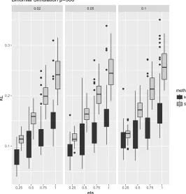
To evaluate the methods, 1000 validation observations are generated from the data generating model and the KL divergence is measured for each of the 50 replications. The KL divergence for a replication is defined as,

1 1000

1000 X

i=1 15 X

k=1

log

b

πik

π∗_ik

b

πik+ log

1−π_bik

1−π∗_ik

(1−_bπik)

,

whereπ_ik∗ is the true probability and _bπk(xi, δ, γ) is the estimated probability for responsek

for validation observation i.

Box plots are presented to compare the KL divergence of MCEN and SEN for the different settings in the case of p = 300. The results of simulation in cases where p = 12 and 100 are available in the supplementary material. Figure 5 presents the KL divergence results from the 50 replications for the different settings of η and λ. In terms of KL divergence MCEN outperforms SEN in all settings.

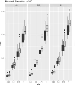
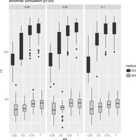
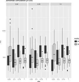
A comparison of MSE of coefficient estimates between methods is shown using box plots in Figure 6 and shows similar results to the cases of p = 12 and 100 available in the supplementary material. The results show that based on MSE binomial MCEN either outperforms or performs as well as binomial SEN. Figures 7 and 8 report the number of true positive and false positive predictors selected by each method for each combination of η and λ when p = 300, and MCEN outperforms SEN by generally selecting more true positive predictors, while the number of false predictors selected varies by the signal size. For smaller signals MCEN selects a smaller number of false predictors, but for larger signals MCEN tends to select more false predictors.

6. Data Example

6.1 Genomics Data

0.02 0.05 0.1

0.25 0.5 0.75 1 0.25 0.5 0.75 1 0.25 0.5 0.75 1

0.1 0.2 0.3

eta

KL

method MCEN

SEN Binomial Simulation p=300

0.02 0.05 0.1

0.25 0.5 0.75 1 0.25 0.5 0.75 1 0.25 0.5 0.75 1

0.01 0.02 0.03

eta

MSE

method MCEN

SEN Binomial Simulation p=300

0.02 0.05 0.1

0.25 0.5 0.75 1 0.25 0.5 0.75 1 0.25 0.5 0.75 1

50 100

eta

TV

method MCEN

SEN Binomial Simulation p=300

0.02 0.05 0.1

0.25 0.5 0.75 1 0.25 0.5 0.75 1 0.25 0.5 0.75 1

500 1000

eta

FV

method MCEN

SEN Binomial Simulation p=300

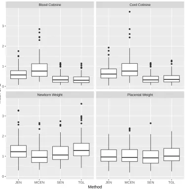
2004), but placental weight is hard to use as a predictor since it is observed at birth. The two measurements of cotinine levels are essentially measuring the same thing and are clearly related to smoking status. Thus we can test if these variables were correctly clustered and smoking status selected in the MCEN models.

The same methods used in Section 5.1 are used to fit the data, except we did not implement the TMCEN method as we did not assume to know the true clustering structure of the response variables. To evaluate the methods we randomly partitioned the data into 50 training and 15 testing samples. All four response variables are modeled on the log scale. In the training data all variables are centered and scaled to have mean zero and a standard deviation of one. We filter the gene expression data for each response by using the top 25 genes in terms of absolute value of correlation with a given response. For the joint modeling methods we use a union of the top 25 genes for each response. Models are fit using the training data, then predictions are evaluated on the testing samples. We compare the methods by looking at the ASPE, as defined in Section 5.1. For MCEN we consider clusters of size 1, 2 and 3. The process is repeated 100 times and the ASPE for all methods and responses are included in Figure 9. The MCEN method performs the best for modeling birth weight, the most clinically interesting variable, and is about the same as the other methods for modeling placenta weight. However, it does worse than the other three methods for modeling cotinine level. In all 100 random partitions the MCEN method correctly grouped the two cotinine responses together and selected smoking status as a predictor for those two responses.

6.2 Concession Data

We analyzed 2000 concession transactions from a major event venue. Each transaction is linked with the customer’s information from the venue’s loyalty program. These data are proprietary and cannot be made publicly available. Whether a customer purchases a specific item, 0 if they do and 1 if they do not, is the response and customer information from the loyalty program, such as seat identification and amount spent on previous concession sales, are treated as the covariates. The multiple response setting comes from there being multiple items available for sale at the concession stands. In total there are 34 predictor variables, stemming from purchase history from the venue, ticketing, and seating. The same customer may appear in the data more than once, but any correlation structure is ignored. We analyze two different sets of responses with the same covariates. The point-of-sale system records purchases in two different item set groupings; menu group (7 items) and food group (12 items). The different groups provide different insights into customer habits as the items form different groups.

Similar to the simulation section we compared SEN and MCEN, with tuning parameter selected as described in Section 5.2. For Q, the number of groups, we consider values of

●

● ●

●

● ● ●

●

● ● ● ● ● ● ● ●

● ●

● ● ● ● ●

● ●

●

●

● ● ●

● ● ● ● ● ● ● ● ●

● ● ●

● ●

●

● ●

●

● ●

● ● ● ●

● ●

● ● ●

●

● ● ●

●

Blood Cotinine Cord Cotinine

Newborn Weight Placental Weight

0 1 2 3

0 1 2 3

JEN MCEN SEN TGL JEN MCEN SEN TGL

Method

Mean SPE

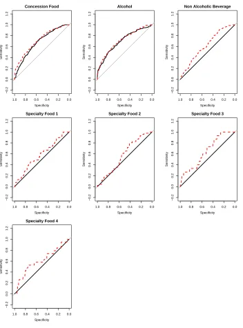
For comparison of the methods we present the ROC curves as a metric for classification performance on the 1000 validation observations. Figure 10 presents the ROC curves and shows that in most situations the binomial logistic MCEN was competitive with SEN. In this analysis MCEN found 3 response clusters where the first cluster contained concession food, the second cluster contained both alcoholic and non-alcoholic beverages, and the third cluster contained all specialty item groups. For comparison we used k-means clustering on the predicted values of the independent elastic net, and selected the number of clusters based on the gap statistic. It selected 2 clusters. The first cluster had concession and both beverage types, while the second cluster contained all specialty items.

The resulting ROC curves for the food group analysis are presented in Figure 11. Five clusters were found by binomial logistic MCEN. The first cluster has popcorn, hamburger, french fires, bottled water, appetizers, and a chicken basket. These correspond to low selling non-alcoholic items. The second cluster consists of hot dogs, craft beer and misc sides, which represents a group of higher selling items. The last three clusters are singleton clusters consisting of non-alcoholic beverages, domestic beer, and liquor. These clusters represent high selling items with different demographics important in each. We also ran k-means clustering on the predicted values from the EN results, and found no distinct clustering using the gap statistic to select the number of clusters. Thus the MCEN method clusters all cold beverages together, while using k-means on fitted values from SEN does not find this clustering. The results of both analyses show that SEN outperforms MCEN using ROC curves. This could be due to the coarseness of MCEN framework, which assumes a similar sparsity structure for all responses. The grouping insights given from the resulting MCEN clusters provide a starting point for investigating each cluster individually with its own MCEN models. This procedure would allow for different levels of sparsity for different clusters. Flexibility such as this should be addressed in extensions of MCEN.

7. Discussion

We present a method for simultaneous estimation of regression coefficients and response clustering for a multivariate response model. The method is introduced for the case of continuous and binary responses. Future work could include extending the model to other GLM settings. Currently, our model imposes the same amount of sparsity on all response models, but this could be relaxed by allowing a sparsity tuning parameter for each individual response or each response group. ThemcenR package that implements the methods outlined in this article is available on CRAN (Sherwood and Price, 2018).

Define`(B) as a likelihood or convex objective function,P(β, Dq) as a distance function

between all elements where PQ

q=1P(B, Dq) is an optimization problem to separate the r

p-dimensional coefficient vectors intoQclusters andpδ(B) as a penalty function with tuning

parameterδ. Then the MCEN method could be generalized to a larger class of estimators where

( ˆB,Dˆ) = arg min

B,D1,...,DQ

`(B) +γ

Q

X

q=1

P(B, Dq) +pδ(B). (32)

One example would be to defineP(B, Dq) as anL1 norm to penalize the difference between

Concession Food

Specificity

Sensitivity

1.0 0.8 0.6 0.4 0.2 0.0

−0.2

0.0

0.2

0.4

0.6

0.8

1.0

1.2

Alcohol

Specificity

Sensitivity

1.0 0.8 0.6 0.4 0.2 0.0

−0.2

0.0

0.2

0.4

0.6

0.8

1.0

1.2

Non Alcoholic Beverage

Specificity

Sensitivity

1.0 0.8 0.6 0.4 0.2 0.0

−0.2

0.0

0.2

0.4

0.6

0.8

1.0

1.2

Specialty Food 1

Specificity

Sensitivity

1.0 0.8 0.6 0.4 0.2 0.0

−0.2

0.0

0.2

0.4

0.6

0.8

1.0

1.2

Specialty Food 2

Specificity

Sensitivity

1.0 0.8 0.6 0.4 0.2 0.0

−0.2

0.0

0.2

0.4

0.6

0.8

1.0

1.2

Specialty Food 3

Specificity

Sensitivity

1.0 0.8 0.6 0.4 0.2 0.0

−0.2

0.0

0.2

0.4

0.6

0.8

1.0

1.2

Specialty Food 4

Specificity

Sensitivity

1.0 0.8 0.6 0.4 0.2 0.0

−0.2

0.0

0.2

0.4

0.6

0.8

1.0

1.2

Hot Dog

Specificity

Sensitivity

1.0 0.6 0.2

−0.5

0.0

0.5

1.0

1.5

Popcorn

Specificity

Sensitivity

1.0 0.6 0.2

−0.5

0.0

0.5

1.0

1.5

Craft Beer

Specificity

Sensitivity

1.0 0.6 0.2

−0.5

0.0

0.5

1.0

1.5

Hamburger

Specificity

Sensitivity

1.0 0.6 0.2

−0.5

0.0

0.5

1.0

1.5

Non Alcoholic Beverage

Specificity

Sensitivity

1.0 0.6 0.2

−0.5

0.0

0.5

1.0

1.5

French Fries

Specificity

Sensitivity

1.0 0.6 0.2

−0.5

0.0

0.5

1.0

1.5

Domestic Beer

Specificity

Sensitivity

1.0 0.6 0.2

−0.5

0.0

0.5

1.0

1.5

Bottled Water

Specificity

Sensitivity

1.0 0.6 0.2

−0.5

0.0

0.5

1.0

1.5

Misc Sides

Specificity

Sensitivity

1.0 0.6 0.2

−0.5

0.0

0.5

1.0

1.5

Liquor

Specificity

Sensitivity

1.0 0.6 0.2

−0.5

0.0

0.5

1.0

1.5

Appetizers

Specificity

Sensitivity

1.0 0.6 0.2

−0.5

0.0

0.5

1.0

1.5

Chicken Basket

Specificity

Sensitivity

1.0 0.6 0.2

−0.5

0.0

0.5

1.0

1.5

advantage of the estimator proposed in this paper is that by defining P(B, Dq) as the L2

norm squared, when the coefficients are fixed, the minimization problem is equivalent to a k-means problem. However, different definitions of P(B, Dq) may not have well studied

clustering algorithms to solve the optimization to define the groupings. One challenge of extending this work would be finding functionsP(B, Dq) that become well defined clustering

problems when B is known or proposing new algorithms for solving P(B, Dq). Otherwise

the two-step algorithm proposed in this paper would not work.

The asymptotics in this paper are limited to consistency of the estimator when groups are known. Zhao and Shojaie (2016) presented an inference framework for a similar esti-mator that uses a fusion penalty and demonstrated that inference is still possible even if the structure of the graph that determines the fusion penalty is not correctly specified. Ex-tending the results provided here to include inference would be of great use to practitioners and a good topic for future research.

Acknowledgments

We would like to thank Dr. Sara van de Geer and an anonymous reviewer for their insightful comments on early versions of this work. We would also like to thank Suzanna Emelio of the University of Kansas and Dr. Nancy McIntyre for their careful editing of our manuscript. This work was also partially sponsored by Big XII Faculty Fellowships from West Virginia University and the University of Kansas.

Appendix

A.1. Proof of Theorem 1

Proof Define

L(B) = 1 2n

n

X

i=1

r

X

c=1

(yic−xTi βc)2+

γ

2n

Q

X

q=1

1

|Dq|

X

l,m∈Dq

||X(β_l−β_m)||2₂.

Forl∈Dq

∂

∂β_lL(B) =−

1

n X

T_{Y −X}T_Xβ

l

+XTX 2γ n|Dq|

X

c∈Dq, c6=l

β_l−β_c.

Thus,

¯

β_l

1 +2γ(|Dq| −1)

|Dq|

−β˙_l− 2γ |Dq|

X

c∈Dq, c6=l

¯

β_c= 0. (33)

Therefore forl, m∈Dq

¯

β_l

1 +2γ(|Dq| −1)

|Dq|

−β˙_l− 2γ |Dq|

X

c∈Dq, c6=l

¯

β_c

− β¯_m

1 +2γ(|Dq| −1)

|Dq|

−β˙_m− 2γ |Dq|

X

c∈Dq, c6=m

¯

β_c

Therefore forl, m∈Dq and l6=m

¯

β_m= ¯β_l+ 1 1 + 2γ

˙

β_m−β˙_l

. (34)

Combining (33) and (34) gives

¯

β_l

1 +2γ(|Dq| −1)

|Dq|

= β˙_l+ 2γ

|Dq|

X

c∈Dq, c6=l

¯

β_l+ 1 1 + 2γ

˙

β_c−β˙_l

= β˙_l+2γ(|Dq| −1)

|Dq|

¯

β_l+ 2γ (1 + 2γ)|Dq|

X

c∈Dq, c6=l

˙

β_c−β˙_l,

which completes the proof.

A.2. Proof of Theorem 2

Proof It is assumed that E(2_ic) = 1 and for c6=kthat E(icik) =ρ. Thus, note that for

any v∈ {1, . . . , r}

Var ¯β_v = Var

 



|Dq|+ 2γ

(1 + 2γ)|Dq|

˙

β_v+ 2γ (1 + 2γ)|Dq|

X

s∈Dq,s6=v

˙

β_s  



= (XTX)−1

(

|Dq| |Dq|+ 4γ+ 4γ2

(1 + 2γ)2_|D

q|2

+ 4ργ(|Dq| −1)

|Dq|+ 2γ|Dq| −2γ

(1 + 2γ)2_|D

q|2

)

.

Define bv=Ps∈Dq,s6=v(β ∗

s−β

∗

v). The squared bias term is then

Eh

E β¯_v

−β∗_v 0

E β¯_v

−β∗_v i

= E

β∗_v+ 2γ (1 + 2γ)|Dq|

bv−β∗v

0

β∗_v+ 2γ (1 + 2γ)|Dq|

bv−β∗v

= 4γ

2

(1 + 2γ)2_|D

q|2

||bv||22.

Letω = Trace

n

XTX−1

o

then MSE of ¯β_v will be smaller than MSE of ˙β_v if

ω

(

|Dq| |Dq|+ 4γ+ 4γ2

(1 + 2γ)2_|D

q|2

+ 4ργ(|Dq| −1)

|Dq|+ 2γ|Dq| −2γ

(1 + 2γ)2_|D

q|2

)

+ 4γ

2

(1 + 2γ)2_|D

q|2

||bv||22

which is equivalent to

γ||bv||22 < ω (

|Dq|(|Dq| −1) +γ|Dq|(|Dq| −1)

−ρ

(|Dq| −1)|Dq|+ 2γ(|Dq| −1)2

)

.

Note that,ω|Dq|(|Dq| −1)(1−ρ)>0 and thus if||bv||22 ≤ω(|Dq| −1){|Dq| −2ρ(|Dq| −1)}

then the MSE of ¯β_v is smaller than the MSE of ˙β_v for anyγ >0. Otherwise, the MSE of ¯β_v

will be smaller for anyγ ∈0, ω|Dq|(|Dq|−1)(1−ρ) ||bv||22−ω(|Dq|−1){|Dq|−2ρ(|Dq|−1)}

. Thus for anyv∈ {1, . . . , r}

then anyγ >0 or any γ sufficiently small will result in ¯β_v having a smaller MSE than ˙β_v. The proof is complete because we can then find aγ sufficiently small that will result in ¯β_v

having a smaller MSE than ˙β_v for all v∈ {1, . . . , r}.

A.3. Proof of Corollary 3

The proof of Corollary 3 is similar to the proof of Theorem 1 and only changes with respect to the expected loss rather than the observed loss.

A.4. Theorem 4

The proof of Theorem 4 will include some new definitions and an alternative formulation of (5). In our proof we use a vectorized version of many of the matrices. Let ˜Y= vec(Y),

˜

β = vec(B), ˜β0 = vec( ´B) and ˜E = vec(E). Define Am,s ∈ Rr, where (m, s) ∈ Dq,

with q_|D1

q| in the mth element, − q

1

|Dq| in the sth element and 0 in all other elements,

ADq ∈ R

|Dq|(|Dq|−1)×r _{as the matrix with row vectors A}

m,s where (m, s) ∈Dq, and AD ≡

AT_D

1, . . . , A

T DQ

T

∈ RPQq=1|Dq|(|Dq|−1)×r_.

Then the objective function from (5) can be restated as

1 2n

h

˜

βT nX˜TX˜ +γ(AD ⊗X)T(AD⊗X)

o

˜

β−2 ˜YTX˜β˜i+δ||β˜||₁

= `( ˜β) +δg( ˜β).

In addition define, ˜`(∆,β˜)≡`( ˜β+∆)−`( ˜β)− h∇`( ˜β,∆)i.

First, we will present some lemmas that are helpful in proving Theorem 4. A general outline of the proof for Theorem 4 is by using the triangle inequality we have ||vec( ¯B−

B∗)||2 ≤ ||vec( ¯B−B´)||2+||β˜ 0

−β˜∗||2. Completing the proof is done by establishing upper

bounds for||vec( ¯B−B´)||2 and||β˜ 0

−β˜∗||2. Much of the proof will require working with ˜β 0

and we introduce the following notation to easily relate ˜β0 and ˜β∗. For responselin group

q defineHl= √_|1 Dq|

P

c∈Dq,c6=lAc,l whereHl∈ R

r _{and H = (H1, . . . ,H}

r)T ∈ Rr×r. Then

we have

˜

β0 =

Ir+

2γ

2γ+ 1H

⊗Ip

˜

For response l is in group q define Ul = _|D1_q|Pk∈Dq(β ∗

k −βl∗) where Ul ∈ Rp and U =

(U1, . . . ,Ur) withU ∈ Rp×r and ˜U= vec(U)∈ Rpr, then

vec

´

B−B∗

2=

2γ

1 + 2γ

(H⊗Ip) ˜β ∗

2 =

2γ

1 + 2γ

˜ U 2. Lemma 5 Under assumption A3

˜

`(∆,β˜0)≥κ||∆||2₂ for all ∆∈ C.

Proof From the definition of ˜`(∆,β˜), assumption A3 and that ∆∈ C it follows that

˜

`(∆,β˜0) = 1 2n∆

Tn_X˜T_{X˜ +γ(A}

D⊗X)T(AD⊗X)

o ∆

≥ 1

2n∆

T_X˜T_X˜∆

≥ κ

2||∆||

2 2.

For any vectora= (a1, . . . , apr)T ∈ Rpr we define the ||a||∞ as theL∞ norm ofa, that

is||a||∞= max

i |ai|.

Lemma 6 For B¯ from (5), under assumptions A1-A4 with δ ≥ 2

∇`( ˜β

0 )

∞ then there

exists a positive constant c3 such that

vec( ¯B−

´ B) 2 2≤9

δ2

κ2s.

Proof Define the set ´S = {j ∈ {1, . . . , rp},β˜0_j 6= 0}. By assumption A5 and Corollary 3 ´S = S, that is ˜β0_j = 0 if and only if ˜β∗_j = 0. Define ψ(M) ≡ sup

u∈M\{0} ||u||1

||u||2. Note that

ψ{M(S)}= √s. Also, note that the dual norm of the L1 norm is the L∞ norm. Results

follow from Theorem 1 of Negahban et al. (2012) and Lemma 5.

Lemma 7 Under the conditions of Theorem 4 there exists positive c1, c2 and c3 such that vec ¯

B−B´

2 ≤ 48σ κ r

slog(rp)

n ,

with probability at least 1−c1exp(−c2nδ2).

Proof If we can find positive constants c1 and c2 such that with probability at least

1−c1exp(−c2nδ2) thatδ ≥2 ∇`( ˜β

0 )

the condition thatδ = 16σ

q log(rp)

n . Note that

2 ∇`( ˜β

0 )

_∞ = 2 1 n hn ˜

XTX˜+γ(AD⊗X)T(AD⊗X)

o

˜

β0−X˜TY˜

i _∞ = 2 1 n n ˜

XTX˜ +γ(AD⊗X)T(AD⊗X)

o

Ir+

2γ

2γ+ 1H

⊗Ip

˜

β∗−X˜T

˜

Xβ˜∗+ ˜E _∞ ≤ 2 2γ n(1 + 2γ)X˜

T_X˜U˜

_∞ + 2 γ

n(AD⊗X)

T_(A

D⊗X) ˜β

∗ ∞ +2

2γ2

n(1 + 2γ)(AD⊗X)

T_(A

D⊗X) ˜U

_∞ + 2 1 n ˜

XTE˜ _∞

.

Next, we will establish upper bounds for the first three terms. Define I(l ∈Dq) to be 1 if

l∈Dq and zero otherwise. Using the definition of ˜U and assumptions A4-A6,

2 2γ n(1 + 2γ)

˜

XTX˜U˜ _∞

= 4γ

1 + 2γ l∈{1max,...,r} 1 nX T_X Q X q=1

I(l∈Dq)

X

k∈Dq

1

|Dq|

(β∗_k−β∗_l)

_∞

≤ 4γ

1 + 2γρmaxl∈{1max,...,r} Q X q=1

I(l∈Dq)

X

k∈Dq

1

|Dq|

(β∗_k−β∗_l)

2 ≤ 4γ

1 + 2γρmax´b.

Using assumptions A4-A6,

2

γ

n(AD⊗X)

T_(A

D⊗X) ˜β

∗

_∞ = 2γ max

l∈{1,...,r} 1 nX

T_X X

k,l∈Dq,k6=l

1

|Dq|

(β∗_k−β_l∗)

_∞

≤ 2γρmax max

l∈{1,...,r} X

k,l∈Dq

1

|Dq|

(β_k∗−β∗_l)

2 ≤ 2γρmax´b.

Note that fora∈Dq andb∈Dq that

Ua−Ub =

1

|Dq|



 X

l∈Dq

β∗_l −β∗_a− X

l∈Dq

β∗_l −β∗_b 



= 1

|Dq|

X

l∈Dq

Therefore 2

2γ2

n(1 + 2γ)(AD⊗X)

T_(A

D⊗X) ˜U

_∞

= 4γ

2

1 + 2γ l∈{1max,...,r} 1 nX T_X Q X q=1

I(l∈Dq)

X

k∈Dq

1

|Dq|

(Uk−Ul)

_∞

= 4γ

2

1 + 2γ l∈{1max,...,r} 1 nX T_X Q X q=1

I(l∈Dq)

X

k∈Dq

1

|Dq|

β∗_l −β∗_{k ∞}

≤ 4γ 2

1 + 2γρmaxl∈{1max,...,r} Q X q=1

I(l∈Dq)

X

k∈Dq

1

|Dq|

β∗_l −β∗_k 2 ≤ 4γ

2

1 + 2γρmax

´

b

≤ 2γρmax´b.

Under assumptions A1 and A2 it follows that

P 1

nX˜

T_E˜

∞ > t

≤2 exp

₋

nt2

2σ2 + log(rp)

. (35)

Thus,

Pnδ≥2

∇`( ˜β

0 ) _∞ o ≥ P

δ≥2

1 n ˜

XTE˜ _∞

+ρmax´b

4γ

1 + 2γ + 2γ+ 2γ

≥ P

δ ≥2

1 n ˜

XTE˜ _∞

+ 8γρmax´b

≥ P

3 16δ ≥

1 n ˜

XTE˜ _∞

≥ 1−2 exp

₋

9nδ2

162_2σ2 + log(rp)

= 1−2 exp

−7

2log(rp)

.

Setc1 = 2 and c2= 7₂ and the proof is complete.

Proof of Theorem 4

Proof Applying the triangle inequality we have

vec

ˆ

β−β∗

2 ≤ vec ˆ

β−β´

2+ ˜

β0−β˜∗

2. (36)

For the second term using the upper bound for γ stated in the conditions for Theorem 4 and assumptions A4 and A5 it follows that

˜

β0−β˜∗

2 =

2γ

1 + 2γ

˜ U 2 ≤ 2γ√s´b≤ 5σ

2ρmax r

slog(rp)