Gradient Estimation with Simultaneous Perturbation and
Compressive Sensing
Vivek S. Borkar [email protected]
Department of Electrical Engineering Indian Institute of Technology Bombay Mumbai 400076, India
Vikranth R. Dwaracherla [email protected]
Department of Electrical Engineering Stanford, USA
Neeraja Sahasrabudhe [email protected]
Department of Mathematical Sciences
Indian Institute of Science Education and Research, Mohali SAS Nagar 140306, India
Editor:Sujay Sanghavi
Abstract
We propose a scheme for finding a “good” estimator for the gradient of a function on a high-dimensional space with few function evaluations, for applications where function evaluations are expensive and the function under consideration is not sensitive in all co-ordinates locally, making its gradient almost sparse. Exploiting the latter aspect, our method combines ideas from Spall’s Simultaneous Perturbation Stochastic Approximation with compressive sensing. We theoretically justify its computational advantages and illus-trate them empirically by numerical experiments. In particular, applications to estimating gradient outer product matrix as well as standard optimization problems are illustrated via simulations.
Keywords: Gradient estimation; Compressive sensing; Sparsity; Gradient descent; Gra-dient outer product matrix.
1. Introduction
Estimating the gradient of a given function (with or without noise) is often an important part of problems in reinforcement learning, optimization and manifold learning. In rein-forcement learning, policy-gradient methods are used to obtain an unbiased estimator for the gradient. The policy parameters are then updated with increments proportional to the estimated gradient (Sutton et. al, 2000). The objective is to learn a locally optimum policy. REINFORCE and PGPE methods (policy gradients with parameter-based exploration) are popular instances of this approach (Zhao et. al, 2012) for details and comparisons, (Grond-man et. al, 2012) for a survey on policy gradient methods in the context of actor-critic algorithms). In manifold learning, various finite difference methods have been explored for gradient estimation (Mukherjee, Wu and Zhou, 2010; Wu et. al, 2010). The idea is to use the estimated gradient to find the lower dimensional manifold where the given
func-c
tion actually lives. Optimization, i.e., finding maximum or minimum of a function, is a ubiquitous problem that appears in many fields wherein one seeks zeroes of the gradient. But the gradient itself might be hard to compute. Gradient estimation techniques prove particularly useful in such scenarios.
A further theoretical justification is facilitated by the results of Austin (2016). In Austin (2016), it was shown that given a connected and locally connected metric probability space (X, d, µ) (i.e.,X is a compact metric space with metricdand µis a probability measure on the Borel σ-algebra of (X, d)), under suitable conditions, any function f :Xn7→R is close (inL1(µn)) to a function on a lower dimensional factor space obtained by averaging out the remaining arguments w.r.t. the corresponding product ofµ(see Austin, 2016, Theorem 1.1). As a special case, a similar fact can be proved for real-values 1-Lipschitz functions on R\Z
with metric| · |n
∞ (see Austin, 2016, Theorem 1.2). This suggests that sparse gradients can
be expected for functions on high dimensional spaces with adequate regularity conditions. Over the years gradient estimation has also become an interesting problem in its own right. One would expect that the efficiency of a given method for gradient estimation also depends on the properties of function f. We consider one such class of problems in this paper. Suppose we have a continuously differentiable function f : Rn 7→ R where n is
large, such that the gradient∇f lives mostly in a lower dimensional subspace. This means that one can throw out most of the coordinates of ∇f in a suitable local basis without incurring too much error. In this case, computing ∂x∂f
i ∀i is clearly a waste of means. If in
addition the function evaluations are expensive, most gradient estimation methods become inefficient. Such is the case, e.g., if a single function evaluation is the output of a large time-consuming simulation. This situation is our specific focus. The problem of expensive function evaluations does not seem to have attracted much attention in machine learning literature, though there has been quite a lot of work on this theme in other communities such as engineering and operations research (Joseph and Murthy, 2017; Xu, Caramanis and Mannor, 2016). Most methods, however, focus on learning a good surrogate for the original function (see Jones, Schonlau and Welch, 1998; Pandita, Bilionis and Panchal, 2016; Shan and Wang, 2010).
To handle the first issue, ideas from compressive sensing can be applied. Compressive sensing theory tells us that an s-sparse vector can be reconstructed from m ∼ slog(n/s) measurements. This means that one does not need the information about ∇f in all n
directions, a much smaller number of measurements would suffice. These ideas are frequently used in signal as well as image processing (see Chan et. al, 2008; Duarte et. al, 2008). To remedy the latter difficulty, we use an idea from Simultaneous Perturbation Stochastic Approximation (SPSA) due to Spall (Spall, 1992), viz., the Simultaneous Perturbation (SP).
We begin by explaining the proposed method for gradient estimation. Important ideas and results from compressive sensing and SPSA that are relevant to this work are discussed in Section 2.1 and Section 2.2 respectively. We state the main result in Section 2.3. Section 3 presents applications to manifold learning and optimization with simulated examples.
Some notational preliminaries are as follows. By k · k1 and k · k we denote the l1 and l2 norms in Rn respectively. By abuse of notation, we also denote the Frobenius norm for
matrices overRbyk · k. Throughout, ‘a.s.’ stands for ‘almost surely’, i.e., with probability
2. Gradient Estimation: Combining Compressive Sensing and SP
As mentioned above, if function evaluations are expensive, SP works well to avoid the problem of computing function multiple times. However, if the gradient is sparse it makes sense to use the ideas of compressive sensing to our advantage. Combining these two techniques helps us overcome the problem of too many function evaluations and also exploit the sparse structure of the gradient. The idea is to use SP to get sufficient number of observations to be able to recover the gradient vial1-minimization. We describe the method
in detail in the following sub-sections.
2.1 Compressive Sensing
Assume that ∇f ∈ Rn is an approximately sparse vector. The idea of compressive sens-ing is based on the fact that typically a sparse vector contains much less information or complexity than its apparent dimension. Therefore one should be able to reconstruct ∇f
with considerable accuracy with much less information than that of ordern. We will make these ideas more precise in the forthcoming discussion on compressive sensing. We state all the results for vectors in Rn. All of these results also hold for vectors over C. We start by
defining what we mean by sparse vectors.
Definition 1 (Sparsity) The support of a vector x∈Rn is defined as:
supp(x) :={j∈[n] :xj 6= 0}.
where [n] ={1,2, . . . , n}. The vectorx∈Rn is calleds-sparse if at mostsof its entries are
nonzero, i.e., if
kxk0 :=card(supp(x))≤s.
We assume that the observed data y ∈ Rm is related to the original vector x ∈
Rn
via Ax =y for some matrix A ∈ Rm×n, where m < n. In other words, we have a linear
measurement process for observing x. The theory of compressive sensing tells us that if
x is sparse, then it can be recovered from y by solving a convex optimization problem. In particular, given a suitable matrix A and appropriate m, the following l1-minimization problem recoversx exactly.
min
z∈Rnkzk1 subject to y=Az (1)
where y = Ax are the m observations. These ideas were introduced by E. Cand´es and T. Tao in their seminal paper on near-optimal signal reconstruction (Cand´es and Tao, 2006). In this paper, the authors proved that the matrices suitable for the recovery need to have what is called the restricted isometry property (RIP). A large class of random matrices satisfy the RIP with quantifiable ‘high probability’ and are therefore suitable for reconstruction via l1-minimization. In particular, subgaussian matrices have been shown
deterministic matrices is of the order of s2 where sis the sparsity. Thus random matrices are a better choice for linear measurement for reconstruction via compressive sensing if one is willing to settle for probabilistic guarantees.
For the scope of this paper, we consider robust recovery options using Gaussian ran-dom matrices, i.e., matrices whose entries are realizations of independent standard normal random variables.
Remark 2 Matrices with more structure such as random partial Fourier matrix or more
generally, bounded orthonormal systems {φi}Ni=1 can also be used as meaurement matrices
for compressive sensing techniques. Given a random draw of such a matrix with associated
constant K0 ≥ 1 (where K0 is the bound on kφik∞), a fixed s-sparse vector x can be
reconstructed via l1-minimization with high probability providedm≥CK02slogn. For more
details on random sampling matrices in compressive sensing (see Foucart and Rauhut, 2013, Chap. 12).
The crucial point here is that it is enough that the given vector is sparse in some basis. A more detailed discussion on various aspects of compressive sensing can be found in Foucart and Rauhut (2013). In real-life situations the measurements are almost always noisy. A more general statement of problem in (1), that takes into account bounded noise in measurement, bounded in norm by η, is given by:
min z∈Rn
kzk1 subject to kAz−yk ≤η (2)
It may also happen that the original vector x is not sparse but is close to a sparse vec-tor. In other words, we would like the reconstruction scheme to be robust and stable. Foucart and Rauhut (2013, Theorem 9.13) gives explicit error bounds for stable and ro-bust recovery where A is a subgaussian matrix. The bound is expressed in terms of
σs(x) := inf{kx−zk : z ∈ Rn is s-sparse}, the distance of x from the nearest s-sparse
vector, and the measurement error. See Cand´es, Romberg and Tao (2006); Cand´es et. al (2005); Kabanava and Rauhut (2015) for more on robust and stable recovery via compres-sive sensing.
We assume that our observationsy = (y1, . . . , ym) are noisy. The following theorem gives an error bound on the reconstruction from noisy measurements using a Gaussian matrix.
Theorem 3 (Theorem 9.20 in (Foucart and Rauhut, 2013)) Letx∈Rnbe as-sparse
vector. Let M ∈ Rm×n be a randomly drawn Gaussian. Assume that noisy measurements
y=M x+ξ are taken with kξk ≤η. If for 0< <1 and someτ >0,
m2
m+ 1 ≥2s
p
log(en/s) +
r
log(−1) s +
τ
√
s
!2
, (3)
then with probability at least 1− every minimizer xˆ of kzk1 subject to kM z−M xk ≤η
satisfies
kx−x∗k ≤ 2η
τ .
2.2 Simultaneous Perturbation Stochastic Approximation
As discussed above we have a fairly good reconstruction of a sparse gradient ∇f given a sufficient number of observations {yi}. However, as mentioned before, the problem often is the unavailability of these observations. Even though observations for ∇f are not readily available, one may computeyi’s using the available information, that is, noisy measurements of the function f. Note that we have, however, assumed that the function evaluations are computationally expensive. We will now address this issue of estimating∇f with low com-putational overheads.
Letei denote theith coordinate direction for 1≤i≤n. We consider the finite difference approximation
∂f(x(k))
∂xi
≈ f(x(k) +δei)−f(x(k)−δei)
2δ
where x(k) = (x1(k), . . . , xn(k)) and δ >0. By Taylor’s theorem, the error of estimation is O(δk∇2f(x(k))k) where ∇2f denotes the Hessian. This estimate requires 2n function
evaluations. Replacing the ‘two sided differences’ (f(x(k) +δei)−f(x(k)−δei))/2 above by ‘one sided differences’ (f(x(k) +δei)−f(x(k))) reduces this ton+ 1, which is still large for large n. Given that we have assumed f to be such that the function evaluations are computationally expensive, an alternative method is desirable. We use the method devised by Spall (Spall, 1992) in the context of stochastic gradient descent, known as Simultaneous Perturbation Stochastic Approximation (SPSA).
Recall the stochastic gradient descent scheme (Borkar, 2008)
x(k+ 1) =x(k) +a(k) [−∇f(x(k)) +M(k+ 1)], (4)
where:
• {M(k)}is a square-integrable martingale difference sequence, viz., a sequence of zero mean random variables with finite second moment satisfying
E[M(k+ 1)|x(m), M(m), m≤k] = 0∀ k≥0,
i.e., it is uncorrelated with the past. We assume that it also satisfies
sup k
E
kM(k+ 1)k2|x(m), M(m), m≤k
<∞, (5)
• {a(k)}are step-sizes satisfying
a(k)>0 ∀k, X
k
a(k) =∞, X
k
a(k)2 <∞. (6)
The term in square bracket in (4) stands for a noisy measurement of the gradient. Un-der mild technical conditions, x(k) can be shown to converge a.s. to a local minimum of
the classical gradient descent with vanishing error (Borkar, 2008). In practice the noisy gradient is often unavailable and one has to use an approximation ∇cf thereof using noisy
evaluations off, e.g., the aforementioned finite difference approximations, which lead to the Kiefer-Wolfowitz scheme. That is where the SP scheme comes in. We describe this next.
Let {∆i(k),1≤i≤n, k≥0} be i.i.d. zero mean random variables such that
• ∆(k) = (∆1(k), . . .∆n(k)) is independent ofM(`), `≤k+ 1.
• P(∆i(k) = 1) =P(∆i(k) =−1) = 1/2.
Then by Taylor’s theorem, we have that for δ >0:
f(x(k) +δ∆(k))−f(x(k))
δ∆i(k)
≈ ∂f
∂xi
(x(k)) +X j6=i
∂f ∂xi
(x(k))∆j ∆i
. (7)
Note that since ∆j’s are i.i.d. zero mean random variables, we have for j6=i,
E
∂f ∂xi
(x(k))∆j ∆i
x(m), M(m), m≤k−1
= 0.
Hence for the purpose of stochastic gradient descent, the second term in (7) acts as a zero mean noise (i.e., martingale difference) term that can be clubbed with M(k+ 1) as martingale difference noise and gets averaged out by the iteration. This serves our purpose, since the above scheme requires only two function evaluations per iterate given by
xi(k+ 1) =xi(k) +a(k)
−f(x(k) +δ∆(k))−f(x(k))
δ∆i(k)
+Mi(k+ 1).
Our idea is to generate∇ff according to the scheme discussed above.
It should be mentioned that Spall also introduced another approximation based on a single function evaluation (see Borkar, 2008, chap. 10). But this suffers from numerical issues due to the ‘small divisor’ problem, so we do not pursue it here.
2.3 Main result
Algorithm 1 Gradient Estimation at some x∈Rn with SP and Compressive Sensing Initialization:
A= (aij)m×n← random Gaussian matrix.
δ← small positive scalar.
• yi`= f(x+δ
m
P
j
∆`
jaj)−f(x)
δ∆` i
for i= 1, . . . , m; `= 1, . . . , k,
where ∆`j are i.i.d. zero mean Bernoulli random variables taking values in {−1,1}.
• Set ¯yi := Pk
`=1yi`
k , i= 1, . . . , m.
•y= (¯y1, . . . ,y¯m) =A∇f(x) +ζwhereζ denotes the bounded error with boundkζk ≤η.
• Solve the l1-minimization problem stated below to obtain ∇ff:
minimizekzk1 subject to kAz−yk ≤η Output: estimated gradient ∇ff(x).
There are several algorithms for thel1-minimization problem that appears in the last step
of the algorithm above. A detailed discussion of these algorithms, including the Homotopy method (used in Section 3 for thel1-minimization step), can be found in Yang et. al (2010) and Foucart and Rauhut (2013, Chap. 15).
The following theorem states that with high probability such an approximation is “close” to the actual gradient.
Theorem 4 Let f :Rn7→R be a continuously differentiable function with bounded sparse
gradient. Then for m ∈N such that it satisfies the bound in (3), 0 < << m1, and given
δ >0(as in (7)) andτ >0 (as in Theorem 3),∇f can be estimated by a sparse vector ∇ff
such that with probability at least 1−m,
k∇ff − ∇fk<
2t τ
where t >2mO(δ).
Proof LetA∈Rm×nbe a Gaussian matrix such that msatisfies (3). Then, following the same idea as in (7), we have:
yi =
f(x+δ
m
P
j=1
∆jaj)−f(x)
δ∆i
= h∇f(x), aii+
X
j6=i
∆jh∇f, aii ∆i
So we get
y=A∇f + ‘error’, (8)
where we quantify the ‘error’ below.
The above computation is carried outktimes independently, keeping the matrixAfixed and choosing the random vector ∆ according to the distribution defined in Section 2.2. The reason for this additional averaging is as follows. The reconstruction in compressive sensing need not give an unbiased estimate, since it performs a nonlinear (minimization) operation. Thus it is better to do some pre-processing of the SP estimate (which is nearly, i.e., modulo the O(δ) term, unbiased) to reduce its variance. We do so by repeating it k times with independent perturbations and taking its arithmetic mean. This may seem to defeat our original objective of reducing function evaluations, but the k required to get reasonable error bounds is not large as our analysis shows later, and the computational saving is still significant (see ‘Remark 5’ below).
Denote by yl the measurement obtained at lth iteration of SP. The error for a single iteration is given by
ηl=
X
j6=1
∆ljh∇f, a1i
∆l
1
+O(δ), . . . ,X
j6=m
∆ljh∇f, ami ∆l
m
+O(δ)
.
Denote by Xijl = ∆
l jh∇f,aii
∆l i
, j 6= i. Xijl are zero-mean conditionally (given past iterates) independent random variables.
The error vector after kiterations is given by
η = 1
k k X l=1 ηl = 1 k k X l=1 X
j6=1
X1lj+O(δ), . . . ,X
j6=m
Xmjl +O(δ)
= 1 k k X l=1 X
j6=1
X1lj+O(δ), . . . ,1 k
k
X
l=1
X
j6=m
Xmjl +O(δ)
. (9)
In order to apply the ideas from compressive sensing as in Theorem 3, we need to have a bound on the errorkηk. This is obtained as follows. Let K >0 be a constant such that the
O(δ) term above is bounded in absolute value byKδ. Kcan, e.g., be a bound onk∇2fkkAk
and t >2mKδ. Then, by Hoeffding’s inequality we have,
P(kηk ≥t) ≤
m X i=1 P 1 k k X l=1 X
j6=i
Xijl +O(δ)
> t/m ≤ m X i=1 P k X l=1 X
j6=i
Xijl
> kt/2m
≤ 2me−
kt2
2m2(m−1)C2.
Choose the number of iterations, k > 2mt32C2 log 2
. Then,
P(kηk ≥t)≤m. (10)
We define∇ff to be the reconstruction of the gradient using mmeasurements. That is, ∇ff
solves the following optimization problem:
min
z∈Rnkzk1 subject to kAz−yk ≤t,
wherey is as in (8). Our claim then follows from the bound in (10) and Theorem 3.
Remark 5 Note that the minimum number of iterations of SP required to obtain a “good”
estimate of∇f is given by
k > 2m 3C2 t2 log
2 ≥ mC 2
2K2δ2 log
2
≥ sC˜
δ2 log
n s log 2 .
for a suitable constant C˜.
The above ∇ff can now be used as an effective gradient in various problems involving
gradients of high-dimensional functions. Three such applications are discussed in the next section.
3. Applications
modifications to existing algorithms to achieve faster convergence. Algorithm 1 described in Section 2.3 is used for gradient estimation.
As mentioned before, there are various algorithms available for carrying out the l1
-minimization. Here we use the homotopy method (see Donoho and Tsaig, 2008; Foucart and Rauhut, 2013; Yang et. al, 2010). Homotopy method solves the quadratically constrained
l1-minimization problem (2) by considering the following l1-regularized least squares
func-tional:
Fλ(x) = 1
2kAz−yk+λkzk1 forλ >0 (11)
The algorithm traces the piece-wise linear and continuous solution pathλ7→xλ and at each step, an element is added or removed from the support set of the current minimizer. If the minimizerx∗ of (1) is unique then the minimizerxλ of (11) converges to x∗. The idea is to start with a large λsuch that the minimizerxλ of (11) is zero and then trace the solution trajectory in the direction of decreasing λ.
We consider a Gaussian matrix A and get y(n) ← A∇f(x(n)) + error as obtained in equation (8). The last step is to obtain ∇ff(x) via l1-recovery from observations y
and Gaussian random matrix A using the homotopy method described above. All the simulations were performed on MATLAB using the available toolbox for l1-minimization.
(Berkeley database: http://www.eecs.berkeley.edu/ yang/software/ l1benchmark/).
Consider a function f :R250007→R given byf(x) =xTM MTx where, M is 25000×
3-dimensional matrix with 3 non-zero elements per column. Let A be a random Gaussian matrix that is used for measurement. We consider m= 50 measurements.
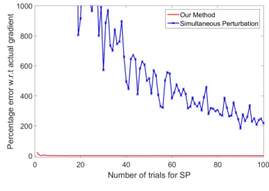
Figure 1 shows the performance of the proposed method with varying number of SP iterations. Figures 2 and 3 show the comparison between our method and naive SP for estimating gradient with gradually increasing number of iterations for averaging over SP (The quantity ‘k’ in (9)). As mentioned earlier, since the gradient is assumed to be sparse, using naive SP to compute derivative in each direction seems wasteful. Although the error diminishes as the number of iterations for SP increase, the proposed method combining compressive sensing with SP consistently performs better.
Figure 1: Percentage error ofk∇f−∇ffkin our method, with varying number of iterations
kfor SP. Here,n= 25000, s= 3 and m= 50.
Figure 2: Performance of the proposed al-gorithm vs. the SP method with varying number iterationskat SP step. Here n = 25000, s = 3 and
m= 50
Figure 4: Performance of the proposed al-gorithm vs. the SP method with varying number iterationskat SP step. Heres= 50 and m= 500.
Figure 5: A closer look at Figure 4: Perfor-mance of the proposed algorithm vs. the SP method with varying number iterations k at SP step. Heres= 50 and m= 500.
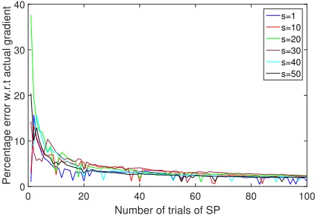
Before we consider specific applications, we illustrate how the percentage error of esti-mated gradient with varyingkfor different sparsity levelss. For appropriately largem, for small k the error is high (this matches with the discussion in Remark 5). As k increases the error is much less. As long as m satisfies (3), the compressive sensing results apply. Figures 6 and 7 show the behaviour of the proposed method with variation in the spar-sity, but with constant number of observations. We consider 10000-dimensional vector with
m = 50 observations. As expected, for a fixed m, as the sparsity increases, increasing k
no longer helps as the compressive sensing results do not apply and the error increases.
f(x) =x(1)2+. . .+x(s)2 was used as a test function for both the simulations.
Number of trials of SP
0 20 40 60 80 100
Percentage error w.r.t actual gradient
0 10 20 30 40
s=1 s=10 s=20 s=30 s=40 s=50
Sparsitys
0 20 40 60 80 100
Percentage error w.r.t actual gradient
20 40 60 80 100 120
Figure 7: Performance of the proposed algorithm with variation in sparsity.
3.1 Manifold Learning: Estimating e.d.r. space
Consider the following semi-parametric model
Y =f(X) +
whereis noise andf is a smooth functionRn7→Rmof the formf(X) =g(bT1X, . . . , bTdX). Define by B the matrix (b1, b2, . . . , bd)T. B maps the data to a d-dimensional relevant subspace. This means that the function f depends on a subspace of smaller dimension given by Range(B) (Note that this is essentially the local view in manifold learning : B can vary with location.). The vectors or the directions given by the vectors bi are called the effective dimension reducing directions or e.d.r. The question is: how to find the matrixB? It turns out that if f doesn’t vary in some direction v, thenv ∈ N ull(EX[G]) where G is the gradient outer product matrix defined as
G= [[Gij]] whereGij =
D∂f
∂xi
(X), ∂f ∂xj
(X)E
andEX[·] denotes the expectation overX. Lemma 1 from (Wu et. al, 2010) stated below implies that to find the e.d.r. directions it is enough to computeEX[G].
Lemma 6 Consider the semi-parametric model
Y =g(bT1X, . . . , bTdX) +, (12)
whererepresents zero mean finite variance noise. Then the expected gradient outer product
(EGOP) matrix G is of rank at most d. Furthermore, if {v1, . . . , vd} are the eigenvectors
associated to the nonzero eigenvalues of G, the following holds:
Clearly, calculating EX[G(X)] is computationally heavy. We therefore try to estimate this matrix. Several methods are known for estimating the EGOP and this has been a very popular problem in statistics for a while. The idea of using EGOP for obtaining e.d.r. originated in Li (1991). While there are other methods based on inverse regression etc., most of the efforts have been directed towards getting an efficient way to estimate gradients in order to finally estimate EGOP (see Xia et. al, 2002). In Mukherjee, Wu and Zhou (2010), the authors use their method of gradient estimation for this purpose. The idea is to use sample observations {f(xi)} for {xi} in a neighborhood of the given point x and minimize overz the error
1
n2
n
X
i,j=1
wij[yi−f(xj)− hz,(xi−xj)i]2,
where wij ≥0 are weights (‘kernel’) that favor locality xi ≈x and are typically Gaussian, with regularization in a reproducing kernel Hilbert space (RKHS). The minimizer then is the desired estimate. In Trivedi et. al (2014) a rather simple rough estimator using directional derivative along each coordinate direction is provided. The authors demonstrate that for the purpose of finding e.d.r., a rough estimate such as theirs suffices. We also propose a method via gradient estimation. TakeGb to be the matrix defined by
b
Gij =
D g∂f
∂xi
,g∂f ∂xj
E
.
In other words,Gb=∇ff∇ff
T
, where∇ff denotes the estimate of∇f obtained by algorithm
1. We impose our previous restrictions onf. That is, the function evaluations at any point are expensive and the gradient off is sparse. In this case we propose an estimate forEX[G] by the mean of Gb over a sample of r points given by the set χ = {(xi, f(xi))}1≤i≤r. By
h · i, we shall denote the empirical mean over the sample setχ. Thus,
hG(X)i= 1
r
X
xi∈χ
∇f(xi)∇f(xi)T
and
hGb(X)i=
1
r
X
xi∈χ
f
∇f(xi)∇ff(xi)T.
Theorem 7 Let f :Rn 7→ Rk from the semi-parametric model in (12) be a continuously
differentiable function with bounded sparse gradient. Then, for 0 < << m1 and some
τ >0, with probability at least 1−m,
EX[G]− hGbi <
6R2
√
r
√
lnn+
r
ln1
!
+2t
τ
2t τ + 2R
where r is the sample size, R is such that k∇fk ≤ R, t is as in Theorem 4 and m ∈N is
The proof closely follows the line of argument in Trivedi et. al (2014).
Proof Note that,
kEX[G(X)]− hGb(X)ik ≤ kEX[G(X)]− hG(X)ik+khG(X)i − hGb(X)ik.
The idea is to bound each term. We use concentration inequality for sum of random matrices (see Trivedi et. al, 2014, Lemma 1) and (Tropp, 2012) for more general results, to claim that for >0,
kEX[G(X)]− hG(X)ik ≤ 6R2
√
r
√
lnn+
r
ln1
!
with probability ≥ 1−. For the second term, it is enough to show that it is bounded for any single sample point x. Observe that for any two vectors v and w, kvvT −wwTk ≤ k(v−w)(v+w)Tk Using this we get, for a fixedx,
kG(x)−Gb(x)k = k∇f(x)∇f(x)T −∇ff(x)∇ff(x)Tk
≤ k∇f(x)−∇ff(x)kk∇f(x) +∇ff(x)k
≤ k∇f(x)−∇ff(x)k
k∇f(x)−∇ff(x)k+ 2k∇f(x)k
≤ 2t
τ
2t τ + 2R
with probability ≥ 1−m, where the last inequality is obtained by applying the bound from Theorem 4.
We now simulate an example to illustrate the decay of the error khG(X)i − hGb(X)ikF
(See Figure 8). Consider a function f :R25000 7→ R3 given by: fi(x) = xTMiMiTx where,
Mi is a 25000-dimensional vector with 3 non-zero elements and fi(x) corresponds to the
ith dimension off(x). A 25000×100 Gaussian random matrix is used for the compressive sensing part of the algorithm. The plot of percentage in normed error betweenhG(X)i and
hGb(X)i, i.e. ||hG(X)i − hGb(X)i||2F is shown below by varying number of samples r = 1 to
0 5 10 15 20 25
Sample size
0 0.5 1 1.5 2 2.5
Percentage of norm of the difference
Figure 8: Percentage error in khG(X)i − hGb(X)ik with number of samples r varying from
1 to 25. Here,n= 25000, s= 3, m= 100 andk= 100.
Figure 9: Comparison of percentage error of khG(X)i − hGb(X)ik computed by plugging
gradient estimates by proposed method vs SGL method. Here, n= 10000, s = 30, m= 100 andk= 100. Number of samples for SGL method are 100.
Learning e.d.r. by estimating the gradient using the method proposed in this paper was compared with the SGL (Sparse Gradient Learning) method proposed in (Mukherjee, Wu and Zhou, 2010) using the same function as above and an exponential kernel (See http:
//www2.stat.duke.edu/~sayan/soft.html for details). This is illustrated in Figure 9.
3.2 Optimization
We consider next a typical problem of function minimization, but only consider a function with sparse gradient. In other words, we want to minimize f(x) where
f :Rn7→R
is a continuously differentiable real-valued Lipschitz function such that function evaluation at a point inRnis typically expensive. We also assume thatnis large and that∇f is sparse.
In addition, we assume that the critical points off (i.e., the zeros of∇f) are isolated. (This is generically true unless there is overparametrization.) The idea is to use the stochastic gradient scheme (4) with the standard assumptions (5), (6). It follows from the theory of stochastic approximation (see Borkar, 2008, chap. 2) that under above conditions, the solution of the random difference equation (4) tracks with probability one the trajectory of the solution of a limiting o.d.e. as long as the iterates remain bounded, which they do under mild additional conditions on f. Following (Borkar, 2008, chap. 2), we use this so called ‘o.d.e. approach’ which states that the algorithm will a.s. converge to the equilibria of the limiting o.d.e., which is
˙
x(t) =−∇f(x(t)). (13) For this,f itself serves as the Lyapunov function, leading to the conclusion that the trajec-tories of (13) and therefore a.s., the iterates of (4) will converge to one of its equilibria, viz., the critical points of f. In fact under additional conditions on the noise, it will converge to a (possibly random) stable equilibrium thereof, viz., a local minimum (ibid., Chapter 4).
The stochastic gradient scheme requires ∇f(x) at each iteration. The problem often is the unavailability of ∇f(x), as already noted. It is therefore important to have a good method for estimating the gradient. Typically one would obtain noisy measurements and hence the estimate will have a non-zero errorη. It is known that if the error remains small, the iterates converge a.s. to a small neighbourhood of some point in the set of equilibria of (13). We analyze the resultant error below. Also, the error obtained in SP is zero-mean modulo higher order terms, so one can even take an empirical average over a few separate estimates in order to reduce variance. For high dimensional problems, the number of function evaluations remains still small as compared with, e.g., the classical Kiefer-Wolfowitz scheme. We use Theorem 4 to justify using SP (Simultaneous Perturbation Stochastic Approximation) combined with compressed sensing to obtain an approximation for the gradient and then use the above scheme to minimizef.
Consider the following stochastic approximation scheme:
xn+1=xn+a(n)[−∇f(xn) +Mn+1+η(n)] (14)
where {η(n)} is the additional error arising due to the error in gradient estimation. That is,∇ff(xn) =∇f(xn)−η(n). If supnkη(n)k< 0 for some small0, then the iterates of (14)
converge to a small neighbourhood A of some pointx∗ inH ={x:∇f(x) = 0} (see Tadic and Doucet, 2017) and (Borkar, 2008, chap. 10)). This is ensured by a Lyapunov argument as follows. The limiting o.d.e. is of the form
˙
for some measurable ˘η(·) withkη˘(t)k ≤0 ∀t. Then d
dtf(x(t)) =−k∇f(x(t))k
2+h∇f(x(t)),η˘(t)i,
which is < 0 as long as k∇f(x(t))k2 > |h∇f(x(t)),η˘(t)i|. Therefore x(t) will converge to
the set
{x:k∇f(x)k ≤0}.
Assume that the Hessian ∇2f(x∗) is positive definite, which is generically so for
iso-lated local minima. Then for A small enough, the lowest eigenvalue λm(x) of ∇2f(x) for x ∈A is >0. By mean value theorem, ∇f(x) =∇2f(x0)(x−x∗) for some x0 ∈A, so
k∇f(x)k ≥λm(x0)kx−x∗k. Thus there is convergence to a ball of radius 0
λm around x
∗.
(A statement to this result without the estimate on the radius of the ball is contained in Theorem 1 of (Hirsch, 1989).) Thus we have:
Theorem 8 The stochastic gradient scheme
xn+1 =xn+a(n)[−∇ff(xn) +Mn+1]
a.s. converges to a ball of radius O(0) centered at some local minimum of f, where ∇ff is
the reconstructed gradient as in Theorem 4 and 0 is a bound onk∇ff− ∇fk.
Proof The claim is immediate from the above observations about the perturbed differential
equation and Theorem 6, pp. 58-59, (Borkar, 2008).
See Tadic and Doucet (2017) for a finer analysis. Also, observe that we have only discussed asymptotic convergence above. For real-life optimization problems, however, we must ensure that the scheme in (14) converges to a neighbourhood of x∗ in finite time. This is indeed true and recent concentration-type results (see Kamal, 2010; Thoppe and Borkar , 2015)) strengthen the theoretical basis for plugging ∇ff(x) in place of ∇f(x) in
stochastic gradient descent schemes. The results in Kamal (2010) involve estimates on lock-in probability, i.e., the probability of convergence to a stable equilibrium given that the iterates visit its domain of attraction. An estimate on the number of steps needed to be within a prescribed neighborhood of the desired limit set with a prescribed probability is also obtained. Specifically, the result states that if the n0th iterate is in the domain of
attraction of a stable equilibrium x∗, then after a certain number of additional steps, the iterates remain in a small tube around the differential equation trajectory converging to x∗
with probability exceeding
1−O e
− C
(P∞m=n 0a(m)2)
1 4
!
,
ipso facto implying an analogous claim for the probability of remaining in a small
formula. We have omitted the details of both the cases as it needs much additional nota-tion to replicate them here. These would, however, apply to the exact stochastic gradient descent. Since we have an additional error due to approximate gradient as in the preceding theorem, we need to combine the results ofibid. with the above theorem to make a weaker claim regarding how small the neighborhood of x∗ in question can be. Furthermore, these claims are about iterates which are in the domain of attraction of a stable equilibrium. This, however, is not a problem, as ‘avoidance of traps’ results as in Section 4.3 of Borkar (2008) (also see Benaim, 1996; Brandi´ere and Duflo, 1996; Pemantle, 1990) ensure that if the noise is rich enough in a certain precise sense, unstable equilibria are avoided with probability one.
Remark 9 Note that the gradient descent is a stochastic approximation scheme which itself
averages out the noise. So in principle the averaging over k steps at the SP stage in the
original algorithm can be skipped. This means that for a stochastic gradient descent scheme, we cut down the cost of function evaluation even further. The simulations in the next section confirm that good results are obtained without averaging over SP iterations. There is, however, a standard trade-off involved between per step computation / speed of convergence, and fluctuations (equivalently, variance) of the estimates: any additional averaging improves the latter at the expense of the former.
3.3 Numerical experiments
We compare following three algorithms.
1. Actual Gradient Descent
This is the classical stochastic gradient descent with exact gradient.
Algorithm 2 Stochastic Gradient Decent with Compressive Sensing
Initialization:
x(0) =xinitial, A←random Gaussian matrix
a(n) be a sequence that satisfies the properties of stepsize listed above.
Iteration: Repeat until convergence criteria is met at n=n#. At nth iteration:
y(n) ←A∇f(x(n)) + error
f
∇f(x(n))←l1− minimization with Homotopy(y(n), A)
x(n+ 1) ←x(n)−a(n)[∇ff(x(n))]
Output: Approximate minimizer of f i.e. x(n#)
HereHomotopy(y(n), A) denotes thel1-recovery from observationsy(n) and Gaussian
2. Accelerated Gradient Method
Accelerated gradient scheme was proposed by Nesterov (Nesterov, 1983). While Gra-dient Descent algorithm has a rate of convergence of order 1/safterssteps, Nesterov’s method achieves a rate of order 1/s2. We implement the method here to achieve an improvement in the time complexity further. The idea is to replace the nth iteration above by the following.
At nth iteration:
y(n) ←A∇f(x(n)) + error
f
∇f(x(n))←l1− minimization with Homotopy(y(n), A)
z(n+ 1) ← x(n)−a(n)[∇ff(x(n))
x(n+ 1) ← (1−γ(n))z(n+ 1) +γ(n)z(n) where, λand γ are as follows:
λ(0) = 0, λ(n) = 1 +
p
1 + 4λ2(n−1)
2 , and γ(n) =
1−λ(n)
λ(n+ 1).
This gives us faster convergence towards the minimum.
3. Adaptive Method
Another way to achieve a faster convergence rate is to perform the l1-minimization adaptively with the gradient descent. The idea is to again use the homotopy method forl1-minimization but this part of the algorithm is run for very few iterations. The
intermediate approximation of∇f is then used for performing the stochastic gradient descent. As expected, the errors are high in the beginning but the convergence is faster.
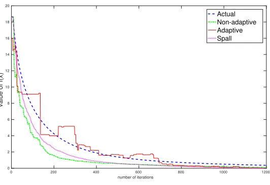
We consider the following function to test our algorithms:
f(x) = (xTM1TM1x)3+ (xTM2TM2x)2+xTM1TM2x (15) where, functionf :Rn7→RandM1, M2 aren×srandom matrices. This is to ensure
sparsity of the gradient. Here, n = 25000 and number of non-zero entries in each column ofM1 and M2 are s= 3. Number of measurements,m= 500. A is an×m
random Gaussian matrix.
0 200 400 600 800 1000 1200 number of iterations
0 2 4 6 8 10 12 14 16 18 20
value of f(x)
Actual Non-adaptive Adaptive Spall
Figure 10: Comparison of Gradient descent with actual gradient ∇f and estimated gra-dient ∇ff using non-adaptive, adaptive schemes and Spall’s SPSA. Here, n =
25000, s= 3 and m= 500
Algorithm Used n = 1000 (sec) n = 10000 (sec) n = 25000 (sec)
Adaptive Method 4.3 62.3 85.4
Without Adaptive 50.572 612.3 1004.5
Spall’s SPSA 25.0 459.8 864.5
Actual Gradient Method 64.1 4641.12 7526
As expected, adaptive method turns out to be faster compared to the non-adaptive method which in turn is much faster than the algorithm that computes actual gradients. Incidentally, the classical scheme all but converges in under 1000 iterations. Even so it takes more time than the other two which take more iterations. This is because of the heavy per iterate computation for the classical scheme. From the above table it is clear that as the dimensionality of the problem increases, adaptive method proves more and more useful compared to the other two algorithms.
We also compared our method with the method proposed in (Mukherjee, Wu and Zhou, 2010) (See Figure 11). The function in (15) is used for the comparison withn= 10000 and
Number of iterations
0 100 200 300 400 500
Value of f(x)
×104
0 2 4 6 8 10
SGL Our Method
Figure 11: Comparison of Gradient descent using estimated gradient from proposed method vs the SGL method proposed in (Mukherjee, Wu and Zhou, 2010). Here, n= 10000, s= 50 and m= 500. Number of samples for the SGL method = 10.
Number of iterations
0 50 100 150 200 250 300 350
Value of f(x)
0 2 4 6 8
Mukherjee Adaptive
Figure 12: Comparison of Gradient descent using estimated gradient from proposed method vs the SGL method proposed in (Mukherjee, Wu and Zhou, 2010). Here, n= 10000, s= 100 andm= 500. Number of samples for the SGL method = 10.
3.3.1 An Example: Longitude Estimation
In this section, we test our method on real data. Gradient estimation technique proposed in this paper is applied on UJIIndoorLoc Data Set (Torres-Sospedra et. al, 2014) to estimate the longitude information from signal strengths of 520 wireless access points. The Data-set has 19937 samples for training and 1111 samples for testing. We assume that longitude
l is linearly dependent on signal strengths of access points x. Let θ ∈ Rn be the vector assigning weights of signal strengths to each access points. Then,l(θ) =θTx. We recoverθ
by minimizing regularizedl1 norm of the error:
f(θ) = M
X
i=1
1
Mklactual−l(θ)k1+λkθk
where, lactual denotes the actual longitude. In this example, M = 19937, n = 520 and
m= 100, wherem is as in theorem 2.3.
Note that we do not have a closed form expression for the gradient off(θ). We compare the proposed method with Spall’s SPSA. Parameters like k (number of trials of SP) and iteration forl1 minimization are chosen so that both methods converge empirically in least
number of iterations. Taking into account the higher error in SPSA, we take number of trials of SP to be 20 for Spall’s SPSA and 10 for our method. Maximum number of iterations in Homotopy method are limited to 50.
Algorithm: Proposed Method Spall’s SPSA
Mean percentage error on training data 5.43 5.54
Mean percentage error on test data 5.55 5.48
Time taken to train (sec) 16.77 84.81
We can see that both methods obtain similar performance but the method proposed in this paper is much faster. Figure 13 shows the training performance of both methods. Figures 14, 15 show percentage error in reconstruction of training and test data respectively. Percentage error is sorted for better visualization.
0 50 100 150 200 250 300 350
Number of iterations 0
1000 2000 3000 4000 5000 6000 7000
f(
)
Proposed Method Spall's SP
0 0.2 0.4 0.6 0.8 1 1.2 1.4 1.6 1.8 2 Number of samples 104
0 5 10 15 20 25 30 35
error percentage
Proposed Method Spall's SP
Figure 14: Sorted percentage error on train data.
0 200 400 600 800 1000 1200 Number of samples
0 5 10 15 20 25 30 35
error percentage
Proposed Method Spall's SP
Figure 15: Sorted percentage error on test data.
4. Concluding remarks
We have proposed an estimation scheme for gradient in high dimensions that combines ideas from Spall’s SPSA with compressive sensing and thereby tries to economize on the number of function evaluations. This has theoretical justification by the results of (Austin, 2016). Our method can be extremely useful when the function evaluation is very expensive, e.g., when a single evaluation is the output of a long simulation. This situation does not seem to have been addressed much in literature. In very high dimensional problems with sparse gradient, computing estimates for partial derivatives in every direction is inefficient because of the large number of function evaluations needed. SP simplifies the problem of repeated function evaluation by concentrating on a singlerandom direction at each step. When the gradient vectors in such cases live in a lower dimensional subspace, it also makes sense to exploit ideas from compressive sensing. We have computed the error bound in this case and have also shown theoretically that this kind of estimation of gradient works well with high probability for the gradient descent problems and in other high dimensional problems such as estimating EGOP in manifold learning where gradients are actually low-dimensional and gradient estimation is relevant. Simulations show that our method works much better than pure SP.
Acknowledgments
References
T. Austin. On the failure of concentration for the `∞-ball. Israel Journal of Mathematics
211(1):221-238, 2016.
S. A. Bandeira, M. Fickus, G. D. Mixon, and P. Wong. The road to deterministic matri-ces with the restricted isometry property. Journal of Fourier Analysis and Applications
19(6):1123-1149, 2013.
M. Benaim, A dynamical system approach to stochastic approximation, SIAM Journal of
Control and Optimization 34(2):437-472, 1996.
O. Brandi´ere and M. Duflo, Les algorithmes stochastiques contourment-ils les pi`eges?,
An-nals de l’Institut Henri Poincar´e 32(3):395-427, 1996.
Vivek S. Borkar. Stochastic Approximation: A Dynamical Systems Viewpoint. Hindustan Book Agency, New Delhi, and Cambridge University Press, Cambridge, UK, 2008.
E. Cand´es and T. Tao. Near optimal signal recovery from random projections: universal encoding strategies? IEEE Transactions on Information Theory, 52(12):5406-5425, 2006.
E. Cand´es, J. Romberg J. and T. Tao. Stable signal recovery from incomplete and inaccurate measurements, Comm. Pure Appl. Math., 59(8):1207-1223, 2006.
E. Cand´es, M. Rudelson, T. Tao and R. Vershynin. Error correction via linear programming.
InProceedings of the 46th Annual IEEE Symposium on Foundations of Computer Science
(FOCS), 295-308, 2005.
L. W. Chan, K. Charan, D. Takhar, K. F. Kelly, R. G. Baraniuk, G. Richard and D. M. Mittleman. A single-pixel terahertz imaging system based on compressed sensing.Applied
Physics Letters, 93(12):121105-121105-3, 2008.
D. L. Donoho and Y. Tsaig. Fast solution of l1-norm minimization problems when the solution may be sparse, IEEE Transactions on Information Theory, 54:4789-4812, 2008.
M. F. Duarte, M. A. Davenport, T. Dharmpal, J. N. Laska, T. Sun, K. F. Kelly and R. G. Baraniuk. Single-pixel imaging via compressive sampling. IEEE Signal Processing
Magazine, 25(2):83-91, March 2008.
S. Foucart and H. Rauhut. A Mathematical Introduction to Compressive Sensing, Birkh¨auser, New York, 2013.
I. Grondman, L. Busoniu, G. A. D. Lopes and R. Babuska. A Survey of actor-critic reinforce-ment learning: standard and natural policy gradients. IEEE Transactions on Systems, Man, and Cybernetics, Part C: Applications and Reviews, 42(6):1291-1307, Nov. 2012.
M. W. Hirsch. Convergent Activation Dynamics in Continuous Time Networks. Neural
Networks, 2(5): 331-349, 1989.
G. Joseph and C. R. Murthy. A Non-iterative Online Bayesian Algorithm for the Recov-ery of Temporally Correlated Sparse Vectors. IEEE Transactions on Signal Processing, 65(20):5510-5525, 2017.
M. Kabanava and H. Rauhut. Analysisl1-recovery with frames and gaussian measurements.
Acta Applicandae Mathematicae, 140(1):173-195, 2015.
S. Kamal. On the convergence, lock-in probability, and sample complexity of stochastic approximation. SIAM Journal on Control and Optimization, 48(8):5178-5192, 2010.
K. C. Li. Sliced inverse regression for dimension reduction.Journal of the American
Statis-tical Association, 86(414):316-327, 1991.
S. Mukherjee, Q. Wu, and D. X. Zhou. Learning gradients on manifolds. Bernoulli, 16(1):181-207, 2010.
Y. Nesterov. A method of solving a convex programming problem with convergence rate
O(1/k2). Soviet Mathematics Doklady, 27(2):372-376, 1983.
P. Pandita, I. Bilionis and J. Panchal. Extending Expected Improvement for High-dimensional Stochastic Optimization of Expensive Black-Box Functions. Journal of Me-chanical Design 138(11):111412, 2016.
R. Pemantle. Nonconvergence to unstable points in urn models and stochastic approxima-tion. Annals of Probability, 18(2):698-712, 1990.
S. Shan and G. Gary Wang. Survey of modeling and optimization strategies to solve high-dimensional design problems with computationally-expensive black-box functions.
Struc-tural and Multidisciplinary Optimization, 41(2), 219, 2010.
J. C. Spall. Multivariate stochastic approximation using a simultaneous perturbation gra-dient approximation.IEEE Transactions on Automatic Control, 37(3):332-341, 1992.
R. S. Sutton, D. McAllester, S. Singh and Y. Mansour. Policy gradient methods for reinforce-ment learning with function approximation. Advances in Neural Information Processing
Systems, 12:1057-1063, MIT Press, 2000.
V. B. Tadic and A. Doucet. Asymptotic bias of stochastic gradient search. The Annals of
Applied Probability 27(6):3255-3304, 2017.
G. Thoppe and V. S. Borkar. A concentration bound for stochastic approximation via Alexeev’s formula.arXiv:1506-08657v2 [math.OC], 2015.
J. Torres-Sospedra, R. Montoliu, A. Martnez-Us, J. P. Avariento, T. J. Arnau, M. Benedito-Bordonau, and J. Huerta. UJIIndoorLoc: A new multi-building and multi-floor database for WLAN fingerprint-based indoor localization problems.Indoor Positioning and Indoor
Navigation (IPIN), 2014 International Conference, 261-270, 2014.
S. Trivedi, J. Wang, S. Kpotufe and G. Shakhnarovich. A consistent estimator of the ex-pected gradient outerproduct. Proceedings of the Thirtieth Conference on Uncertainty in
J. A. Tropp. User-friendly tail bounds for sums of random matrices. Foundations of
Com-putational Mathematics, 12(4):389-434, 2012.
Q. Wu, J. Guinney, M. Maggioni and S. Mukherjee. Learning gradients : predictive models that infer geometry and statistical dependence. Journal of Machine Learning Research, 11(1922):2175-2198, 2010.
Y. Xia, H. Tong, W. Li, and L.-X. Zhu. An adaptive estimation of dimension reduction space.
Journal of the Royal Statistical Society: Series B (Statistical Methodology), 64(3):363-410,
2002.
H. Xu, C. Caramanis and S. Mannor. Statistical optimization in high dimensions.Operations
research, 64(4):958-979, 2016.
A. Yang, A. Ganesh, S. Sastry, and Y. Ma. Fast l1-minimization algorithms and an
appli-cation in robust face recognition: a review.ICIP, 2010.