Learning Non-Stationary Dynamic Bayesian Networks
Joshua W. Robinson [email protected]
Alexander J. Hartemink [email protected]
Department of Computer Science Duke University
Durham, NC 27708-0129, USA
Editor: Zoubin Ghahramani
Abstract
Learning dynamic Bayesian network structures provides a principled mechanism for identifying conditional dependencies in time-series data. An important assumption of traditional DBN struc-ture learning is that the data are generated by a stationary process, an assumption that is not true in many important settings. In this paper, we introduce a new class of graphical model called a non-stationary dynamic Bayesian network, in which the conditional dependence structure of the under-lying data-generation process is permitted to change over time. Non-stationary dynamic Bayesian networks represent a new framework for studying problems in which the structure of a network is evolving over time. Some examples of evolving networks are transcriptional regulatory networks during an organism’s development, neural pathways during learning, and traffic patterns during the day. We define the non-stationary DBN model, present an MCMC sampling algorithm for learning the structure of the model from time-series data under different assumptions, and demonstrate the effectiveness of the algorithm on both simulated and biological data.
Keywords: Bayesian networks, graphical models, model selection, structure learning, Monte Carlo methods
1. Introduction
A principled mechanism for identifying conditional dependencies in time-series data is provided through structure learning of dynamic Bayesian networks. An important requirement of this learn-ing is that the time-series data is generated by a distribution that does not change with time—it is stationary. The assumption of stationarity is adequate in many situations since certain aspects of data acquisition or generation can be easily controlled and repeated. However, other interesting and important circumstances exist where that assumption does not hold and potential non-stationarity cannot be ignored.
learn-ing algorithm based upon dynamic Bayesian networks that relaxes the data stationarity assumption would be ideally suited to this problem.
As another example, structure learning of DBNs has been used widely in reconstructing tran-scriptional regulatory networks from gene expression data (Friedman et al., 2000; Hartemink et al., 2001). But during development, these regulatory networks are evolving over time, with certain con-ditional dependencies between gene products being created as the organism develops, and others being destroyed. As yet another example, one can use a DBN to model traffic flow patterns. The roads upon which traffic passes do not change on a daily basis, but the dynamic utilization of those roads changes daily during morning rush, lunch, evening rush, and weekends.
If one collects time-series data describing the levels of gene products in the case of transcrip-tional regulation, traffic density in the case of traffic flow, or neural activity in the case of neural information flow, and attempts to learn a DBN describing the conditional dependencies in the time-series, one could be seriously misled if the data-generation process is non-stationary.
Here, we introduce a new class of graphical model called a non-stationary dynamic Bayesian network (nsDBN), in which the conditional dependence structure of the underlying data-generation process is permitted to change over time. In the remainder of the paper, we introduce and define the nsDBN framework, present a simple but elegant algorithm for efficiently learning the structure of an nsDBN from time-series data under a variety of different assumptions, and demonstrate the effectiveness of these algorithms on both simulated and experimental data.
1.1 Related Work
Representing relationships or statistical dependencies between variables in the form of a network is a popular technique in many communities, from economics to computational biology to soci-ology. Recently, researchers have been interested in elucidating the temporal evolution of genetic regulatory networks (Arbeitman et al., 2002; Luscombe et al., 2004) and neural information flow networks (Smith et al., 2006), but were forced to perform their analysis on subsets of the data since their structure learning algorithms assumed stationarity of the data. Additionally, some economics techniques require prior specification of a graphical model (for a particular data set) and assume it is stationary (Carvalho and West, 2007) when the data set may actually be highly non-stationary (Xuan and Murphy, 2007). Therefore, the identification of non-stationary behavior in graphical models is of significant interest and importance to many communities.
We divide models of evolving statistical dependencies into those that model changing structures and those that model changing parameters, and describe examples of both in this section. Addition-ally, we briefly explain how our approach compares and some of the advantages it provides over other methods.
1.1.1 STRUCTURAL NON-STATIONARITY
Approaches that learn structural non-stationarities are those that explicitly model the presence of statistical dependencies between variables and allow them to appear and disappear over time (e.g., they define directed or undirected networks whose edges change over time).
(Han-neke and Xing, 2006). The tERGM model was further extended to the hidden tERGM (htERGM) to handle situations where the networks are latent (unobserved) variables that generate observed time-series data (Guo et al., 2006, 2007).
While the transition model of an htERGM allows for nearly unlimited generality in characteriz-ing how the network structure changes with time, it is restricted to functions of temporally adjacent network structures. Therefore, an evolutionary process that differs between early observations and later observations may not be effectively captured by a single transition model. Also, the emission model defined in Guo et al. (2007) must be estimated a priori and only captures pairwise corre-lations between variables; more complicated recorre-lationships between multiple variables that change over time may be missed altogether. Finally, Guo and colleagues focus on identifying undirected edges. Although it is possible to adapt the ERGM model for directed graphs, it becomes more difficult to define the parameters of the tERGM and the emission model assuming directed edges.
In the continuous domain, some research has focused on learning the structure of a time-varying undirected Gaussian graphical model (Talih and Hengartner, 2005). These authors use a reversible-jump MCMC approach to estimate the time-varying variance structure of the data. They explicitly model the network’s edges as non-zeroes in the precision matrix. While this model allows for fast, efficient sampling, it only does so by defining several restrictions to the model space. First, the structural evolutionary process is piecewise-stationary and restricted to single edge changes. Rapid and significant structural changes would be approximated by a slowly changing network structure, resulting in an inaccurate portrayal of the true evolutionary behavior of the data-generating process. Additionally, the total number of segments or epochs in the piecewise stationary process is assumed known a priori, thereby limiting application of the method in situations where the number of epochs is not known. Finally, this approach only identifies undirected edges (correlations), while time-series data should allow one to identify directed edges (conditional dependencies).
A similar algorithm—also based on undirected Gaussian graphical models—has been devel-oped to segment multivariate time-series data (Xuan and Murphy, 2007). This approach iterates between a convex optimization for determining the graph structure and a dynamic programming algorithm for calculating the segmentation. This results in some notable advantages over Talih and Hengartner (2005): it has no single edge change restriction and the number of segments is calcu-lated a posteriori. The main restriction, however, is that the graph structure must be decomposable. Additionally, because this method models structure as non-zeroes in the precision matrix, it only identifies undirected edges. Finally, the networks (precision matrices) in each segment are assumed independent, preventing the sharing of parameters and data between segments.
1.1.2 PARAMETERNON-STATIONARITY
Approaches that learn parameter non-stationarities are those that explicitly model the evolution of parameters over time. Here we only focus on a few that can be represented as networks with temporally changing parameters.
Switching state-space models (SSMs) represent a piecewise-stationary extension of linear dy-namic systems (Ghahramani and Hinton, 2000). In an SSM, a sequence of observations is modeled as a function of several independent hidden variables which is itself controlled by a switch vari-able. The hidden variables as well as the switch variable all have Markovian dynamics. While this approach is similar to ours in that it describes the evolution of a piecewise-stationary process, it does have some notable differences. Our model has no hidden variables, only observed variables. Critically, our variables are not assumed to be independent; rather, their dependencies are unknown and must be estimated a posteriori. Additionally, the piecewise-stationary process in our approach does not follow Markovian dynamics, like the switch variable in an SSM.
A more closely related model is the recently published non-homogeneous Bayesian network (Grzegorczyk et al., 2008). In this model, the conditional distributions of the variables are assumed to follow a mixture of Gaussians. Each observation is allocated to a single mixture component where the parameters and number of the mixture components are determined a posteriori using an allocation sampler. Unfortunately, an allocation sampler does not allow data to be shared across different mixture components since they are assumed independent. However, this model seems to do a good job of capturing the non-stationary behavior of parameters in a Gaussian Bayesian network, assuming that the underlying structure is inferred correctly.
1.1.3 OURAPPROACH
Although we provide more detail in Section 3, for the purpose of comparison, we define our ap-proach as the identification of a discrete Bayesian network that evolves according to a piecewise-stationary process where edges are gained and lost over time. Building on the Bayesian network model allows us to identify directed networks and results in efficient learning (under certain as-sumptions). Additionally, when the conditional probability distributions of the Bayesian network are multinomial, we can identify linear, non-linear, and combinatorial interactions between vari-ables. Finally, the piecewise-stationary assumption (and additional constraints on how and when edge changes occur) allows our method to scale to large data sets with many variables and provides a natural parameterization for placing priors on the structural evolution process.
Our method falls into the category of models that identify non-stationarities in structure, not parameters. In the rest of this paper, we define non-stationarities as times at which conditional dependencies between variables are gained or lost (i.e., edges are gained or lost). We have chosen to focus on structural non-stationarity for several reasons. First, we are not as interested in making predictions about future data (such as might be the case with spam prediction) as we are in the analysis of collected data to identify non-stationary statistical relationships between variables in multivariate time-series. Additionally, the problems we analyze in this paper are highly multimodal in the posterior over structures and likely to be even more varied in the posterior over parameters. By assuming conjugate parameter priors, we address both problems by averaging out all possible parameters and only examining the posterior over structures.
a structural change, while other changes may be dramatic, yet not alter the structure. Ultimately, a trade-off must be made between simplifying model assumptions resulting in greater statistical power versus a completely general framework requiring approximation schemes. Under our modeling assumptions, we can identify non-stationarities in the parameters of the conditional distributions that are significant enough to result in structural changes; we assume other changes are small enough to not alter edges in the predicted structure.
2. Brief Review of Structure Learning of Bayesian Networks
Bayesian networks are directed acyclic graphical models that represent conditional dependencies between variables as edges. They define a simple decomposition of the complete joint distribution— a variable xi is conditionally independent of its non-descendants given its parents. Therefore, the
joint distribution of every variable xi can be rewritten as P(x1, . . . ,xn) =∏iP(xi|πi), whereπi are
the parents of xi. Bayesian networks may be learned on time-series data, but the semantics are
slightly different, leading to the dynamic Bayesian network (DBN) model. DBNs enable cyclic dependencies between variables to be modeled across time. DBNs are a special case of Bayesian networks, with modeling assumptions regarding how far back in time one variable can depend on another (minimum and maximum lag), and constraints placed on edges so that they do not go backwards in time. For notational simplicity, we assume hereafter that the minimum and maximum lag are both 1.
The task of inferring the structure (i.e., the set of conditional dependencies) of a Bayesian net-work is typically expressed using Bayes’ rule, where the posterior probability of a given netnet-work structure G (i.e., the set of conditional dependencies) after having observed data D is given by
P(G|D) =P(D|G)P(G) P(D) .
Since P(D) is the same for all structures, we see that P(G|D)∝P(D|G)P(G). The prior over networks P(G)can be used to incorporate prior knowledge about the existence of specific edges (Bernard and Hartemink, 2005) or the overall topology of the network (e.g., sparse); often, prior knowledge is not available and P(Θ)is assumed uniform. The marginal likelihood P(D|G)is further defined in terms of the parametersΘiof the conditional probability distributions (CPDs) between a
variable and its parents P(xi|πi,Θi). The entire set of parametersΘifor all variables is simplyΘ.
P(D|G) =
Z
P(D|Θ,G)P(Θ|G)dΘ. (1)
One might be interested in inferring the values of Θ given a particular network, but we will be focusing on learning the network itself, or the set of conditional dependencies. In computer science, this task is often referred to as structure learning; in statistics, it is often called model selection. More detailed reviews of structure learning of Bayesian networks can be found in Buntine (1996), Chrisman (1998), Krause (1998), and Murphy (2001).
2.1 Evaluating the Marginal Likelihood P(D|G)
Evaluation of the marginal likelihood in Equation (1) can be performed either approximately or exactly. The marginal likelihood can be approximated with the Akaike information criterion (AIC), the Bayesian information criterion (BIC) (Friedman et al., 1998), or the minimum description length (MDL) (Lam and Bacchus, 1994; Suzuki, 1996) metric. Each of these metrics suggests how model complexity should be penalized. For example, the AIC metric penalizes free parame-ters less strongly than the BIC metric; therefore, a Bayesian network learned using the AIC metric would be likely be more dense than a Bayesian network learned using the BIC metric.
Alternatively, if a conjugate prior is placed onΘ which is then marginalized out, the value of P(D|G)can be computed exactly. Assuming thatΘparameterizes multinomially distributed condi-tional probability distributions, one can place a conjugate Dirichlet prior on the parametersΘand then marginalize them out to obtain the Bayesian-Dirichlet (BD) metric. The BD metric can be further modified so that all of the networks that represent the same set of conditional independence relationships have the same probability; this is called the Bayesian-Dirichlet equivalent (BDe) met-ric (Heckerman et al., 1995). By using a Dimet-richlet prior and marginalizing over all values ofΘ, the BD and BDe metrics inherently penalize more complex models, so a prior on the network P(G) may not always be necessary. The primary advantage of the BD family of metrics is that the evalu-ation of P(D|G)is exact and can be computed in closed form. However, if the assumption that the parameters of CPDs are multinomially distributed is incorrect, these metrics might not find the true network of conditional dependencies.
Since we will be modifying it later in this paper, we show the closed-form expression for the BDe metric below:
P(D|G) =
n
∏
i=1qi
∏
j=1Γ(αi j) Γ(αi j+Ni j)
ri
∏
k=1Γ(αi jk+Ni jk) Γ(αi jk)
(2)
where qi is the number of configurations of the parent setπi, ri is the number of discrete states
of variable xi, Ni jk is the number of times xi took on the value k given the parent configuration j,
Ni j=∑rki=1Ni jk, andαi j andαi jk are Dirichlet hyper-parameters on various entries inΘ. Ifαi jk is
set toα/(qiri)(essentially a uniform Dirichlet prior), we get a special case of the BDe metric: the
uniform BDe metric (BDeu), whose parameter priors are all controlled by a single hyperparameter
α.
2.2 Deciding Between Search or Sampling Strategies
Once a form of the marginal likelihood P(D|G)is defined and a method for evaluating it is chosen, one must decide whether the objective is to identify the best network or to capture the uncertainty over the space of all posterior networks. Search methods may be used to find the best network or set of networks (i.e., a mode in the space of all networks), while sampling methods may be used to estimate posterior quantities from the space of all networks.
Search methods may be exact or heuristic, but exact search for Bayesian networks is compu-tationally infeasible for more than about 30 variables because the number of possible networks is super-exponential in the number of variables. In fact, identifying the highest scoring Bayesian network has been shown to be NP-Hard (Chickering et al., 1994). If the maximum number of parents for any variable is limited to some constant pmax, the total number of valid networks
simulated annealing (Heckerman et al., 1995), the K2 algorithm (Chickering et al., 1995), genetic al-gorithms (Larra˜naga et al., 1996), and even ant colony optimization (de Campos et al., 2002). Most heuristic searches perform well in a variety of settings, with greedy hill-climbing and simulated annealing being the most commonly used techniques.
A different approach from search is the use of sampling techniques (Madigan et al., 1995; Giu-dici et al., 1999; Tarantola, 2004). If the best network is all that is desired, heuristic searches will typically find it more quickly than sampling techniques. However, sampling methods allow the probability or importance of individual edges to be evaluated over all possible networks. In set-tings where many modes are expected, sampling techniques will more accurately capture posterior probabilities regarding various properties of the network. The primary disadvantage of sampling methods in comparison to search methods is that they often take longer before accurate results become available.
A common sampling technique often used in this setting is the Metropolis-Hastings algorithm, which is a Markov chain Monte Carlo (MCMC) method. The M-H acceptance probability for moving from state x to state x′ is shown below, where each state is a DBN.
α(x,x′) =min
1,p(D|x ′)
p(D|x) ×
p(x′→x)
p(x→x′)
=min
1, p(D|x ′)
p(D|x)
| {z } likelihood ratio
× ∑M′p(M
′)p(x|x′,M′)
∑Mp(M)p(x′|x,M)
| {z }
proposal ratio (3)
where M is the move type that allows for a transition from state x to x′ and M′ is the reverse move type for a transition from state x′ back to state x. While multiple moves may result in a transition from state x to state x′ (and vice versa), typically there is only a single move for each transition. In such a case, the sums over M and M′each only include one term, and the proposal ratio can be split into two terms: one is the ratio of the proposal probabilities for move types and the other is the ratio of selecting a particular state given the current state and the move type. The choice of scoring metric determines the likelihoods, and p(M′) and p(M)are often chosen a priori to be equivalent or simple to calculate.
2.3 Determining the Move Set
Once a search or sampling strategy has been selected, one must determine how to move through the space of all networks. A move set defines a set of local traversal operators for moving from a particular state (i.e., a network) to nearby states. The set of states that can be reached from the current one is often called the local neighborhood of that state. The values of p(x′|x,M)and
p(x|x′,M)in the proposal ratio are defined by the move set.
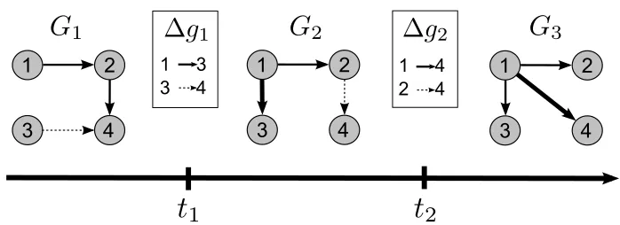
Figure 1: An example nsDBN with labeled components (namely, transition times t1and t2and edge change sets∆g1and∆g2). Edges that are gained from the previous epoch are shown as thicker lines and edges that will be lost in the next epoch are shown as dashed lines. Note that the network at each epoch is actually a DBN drawn in compact form, where each edge represents a statistical dependence between a node at time t and its parent at the previous time t−1.
3. Learning Non-Stationary Dynamic Bayesian Networks
While DBNs are excellent models for describing dependencies between time-series random vari-ables, they cannot represent or reason about how these dependencies might change over time. In contrast, our nsDBN model is capable of characterizing dependencies between temporally observed variables, as well as reasoning about whether and how those dependencies change. Because DBNs are well studied and well understood, we have chosen to introduce the details of our nsDBN model by building upon the existing DBN model. Therefore, we use this section to detail how the structure learning procedure for DBNs needs to be modified and extended to account for non-stationarity when learning a non-stationary DBN.
Assume that we observe the state of n random variables at N discrete times. Call this multivari-ate time-series data D, and further assume that it is genermultivari-ated according to a non-stationary process, which is unknown. The process is non-stationary in the sense that the network of conditional de-pendencies prevailing at any given time is itself changing over time. We call the initial (dynamic) network of conditional dependencies G1 and subsequent networks are called G2,G3, . . . ,Gm. We
define∆gi to be the set of edges that change (either added or deleted) between Gi and Gi+1. The
number of edge changes specified in∆giis si. We define the transition time tito be the time at which
Giis replaced by Gi+1in the data-generation process. We call the period of time between consecu-tive transition times—during which a single network of conditional dependencies is operaconsecu-tive—an epoch. So we say that G1prevails during the first epoch, G2prevails during the second epoch, and so forth. We will refer to the entire series of prevailing networks as the structure of the nsDBN. Figure 1 shows an example nsDBN with the components labeled.
3.1 Updating the Marginal Likelihood and Incorporating Priors
to find the networks G1and G2that have the highest probability given the observed time-series data D and prior. Thus, we want to find the networks that maximize the expression below:
P(G1,G2|D,t1) =P(D|G1,G2,t1)P(G1,G2|t1)
P(D|t1) ∝P(D|G1,G2,t1)P(G1,G2|t1).
To maximize the marginal likelihood P(D|G1,G2,t1)in the above expression, one approach might be to estimate a different network for each epoch. Unfortunately, if the number of observations in each epoch is small, accurate reconstruction of the correct structure may be difficult or impossible (Friedman and Yakhini, 1996; Smith et al., 2003). Additionally, learning each network separately might lead to predictions that are vastly different during each epoch. If prior knowledge about the problem dictates that the networks will not vary dramatically across adjacent epochs, information about the networks learned in adjacent epochs can be leveraged to increase the accuracy of the network learned in the current epoch.
Expanding the simple formulation to multiple epochs, assume there exist m different epochs with transition times T ={t1, . . . ,tm−1}. The network Gi+1 prevailing in epoch i+1 differs from network Giprevailing in epoch i by a set of edge changes we call∆gi. We would like to determine
the sequence of networks G1, . . . ,Gmthat maximize the posterior given below:
P(G1, . . . ,Gm|D,T)∝P(D|G1, . . . ,Gm,T)P(G1, . . . ,Gm|T). (4)
Since each network differs from the previous one by a set of edge changes, we can rewrite the prior and obtain the expression below:
P(G1, . . . ,Gm|T) =P(G1,∆g1, . . . ,∆gm−1|T).
By writing the objective function this way, we rephrase the problem as finding the initial network and m−1 sets of edge changes that best describe the data. Unfortunately, the search space for finding the best structure is still super-exponential (in n) for the initial network and the task of identifying the other networks is exponential (in both m and n). However, using this formulation, it is easy to place some constraints on the search space to reduce the number of valid structures. If we specify that the maximum number of parents for any variable is pmax and, through priors, require
that the maximum number of edge changes for any∆giis smax, the search space for finding the best
structure becomes exponential (in n) for the initial network and exponential (in m and smax) for the
other networks.
We assume the prior over networks can be further split into components describing the initial network and subsequent edge changes, shown below:
P(G1,∆g1, . . . ,∆gm−1|T) =P(G1)P(∆g1, . . . ,∆gm−1|T). leading to the final form of the posterior
structure. First, we assume that the networks evolve smoothly over time. To encode this prior knowledge, we place a truncated geometric prior with parameter p=1−e−λs on the number of
changes (si) in each edge change set (∆gi), with the distribution truncated for si >smax. For the
problems we explore, the truncation has no noticeable effect since smaxis chosen to be large. The
updated posterior for the structure is given below:
P(G1,∆g1, . . . ,∆gm−1|D,T) ∝ P(D|G1, . . . ,Gm,T)
∏
i1−e−λs e−λssi
1− e−λssmax+1
∝ P(D|G1, . . . ,Gm,T)
∏
i
e−λssi
∝ P(D|G1, . . . ,Gm,T)e−λss,
where s=∑isi. Therefore, a (truncated) geometric prior on each si is essentially equivalent to a
(truncated) geometric prior on the sufficient statistic s, the total number of edge changes.
When the transition times are a priori unknown, we would like to estimate them. The posterior in this setting becomes
P(G1,∆g1, . . . ,∆gm−1,T|D) ∝ P(D|G1, . . . ,Gm,T)P(G1,∆g1, . . . ,∆gm−1,T) = P(D|G1, . . . ,Gm,T)P(G1)P(∆g1, . . . ,∆gm−1,T) = P(D|G1, . . . ,Gm,T)P(G1)P(∆g1, . . . ,∆gm−1)P(T). We assume that the joint prior over the evolutionary behavior of the network and the locations of transition times can be decomposed into two independent components. We continue to use the previous geometric prior with parameter p=1−e−λs on the total number of edge changes. Any
choice for P(T)can be made, but for the purposes of this paper, we have no prior knowledge about the transition times; therefore, we assume a uniform prior on T so that all settings of transition times are equally likely for a given value of m.
Finally, when neither the transition times nor the number of epochs are known a priori, both the number and times of transitions must be estimated a posteriori. If prior knowledge dictates that the networks evolve slowly over time (i.e., a transition does not occur at every observation), we can include this knowledge by placing a non-uniform prior on m, for example a (truncated) geometric prior with parameter p=1−eλm on the number of epochs m, with the distribution truncated for
m>N. A geometric prior on the number of epochs is equivalent to a geometric prior on epoch lengths (see Appendix A).
The form of the geometric prior was chosen for convenience since under a log transformation, the likelihood (and prior) calculations reduce to: log(likelihood)−λss−λmm. In general, large
values ofλmencode the strong prior belief that the structure changes slowly (i.e., few epochs exist)
and large values ofλs encode the strong prior belief that the structure changes smoothly (i.e., few
edge changes exist).
Fortunately, the likelihood component of the posterior does not change whether we know the transition times a priori or not. Therefore, any uncertainty about the transition times can be incor-porated into the evaluation of the prior, leaving the evaluation of the likelihood unchanged.
3.2 Evaluating the New Marginal Likelihood
can be modified to account for non-stationarity, but we chose to extend the BDe metric because it is exact and because edges are the only representation of conditional dependencies that are left after the parameters have been marginalized away. This provides a useful paradigm for non-stationarity that is both simple to define and easy to analyze.
The BDe metric needs to be modified when learning an nsDBN because in Equation (2), Ni j
and Ni jkare calculated for a particular parent set over the entire data set D. However, in an nsDBN,
a node may have multiple parent sets operative at different times. The calculation for Ni j and Ni jk
must therefore be modified to specify the intervals during which each parent set is operative. Note that an interval may include several epochs. An epoch is defined between adjacent transition times while an interval is defined as the union of consecutive epochs during which a particular parent set is operative (which may include all epochs).
For each node i, the parent setπiin the BDe metric is replaced by a set of parent setsπih, where
h indexes the interval Ihduring which parent setπihis operative for node i. Letting pibe the number
of such intervals and qihbe the number of configurations ofπihresults in the expression below:
P(D|G1, . . . ,Gm,T)∝ n
∏
i=1pi
∏
h=1qih
∏
j=1Γ(αi j(Ih)) Γ(αi j(Ih) +Ni j(Ih))
ri
∏
k=1Γ(αi jk(Ih) +Ni jk(Ih)) Γ(αi jk(Ih))
where the counts Ni jkand pseudocountsαi jk have been modified to apply only to the data in each
interval Ih. The modified BDe metric will be referred to as nsBDe. Given that |Ih|=th+1−th,
we set αi jk(Ih) = (αi jk|Ih|)/N (e.g., proportional to the length of the interval during which that
particular parent set is operative). Ifαi jkis set everywhere toα/(qiri)as in the BDeu metric, then
we generalize the BDeu metric to nsBDeu, and the parameter priors are again all controlled by a single hyperparameterα.
The derivation of the BDe metric requires seven assumptions: multinomial sample, parameter independence, likelihood modularity, parameter modularity, Dirichlet distribution for parameters, complete data, likelihood equivalence, and structure possibility (Heckerman et al., 1995). To ex-tend the BDe metric to account for non-stationary behavior, we must exex-tend only the parameter independence assumption.
Parameter independence is split into local parameter independence and global parameter inde-pendence. Letting G represent an individual network, global parameter independence is represented as p(ΘG|G) =∏ni=1p(Θi|G). In other words, the conditional probabilities can be decomposed by
variable. Local parameter independence is represented as p(Θi|G) =∏qj=i 1p(Θi j|G); the conditional
probabilities for each variable are decomposable by parent configuration.
For nsDBNs, we also need to assume parameter independence across intervals. Parameter in-dependence is thus split into three assumptions. The updated parameter inin-dependence assumptions are defined below, whereGrepresents an nsDBN structure, or set of networks.
Global parameter independence: The conditional probabilities are decomposable by variable:
p(ΘG|G) = n
∏
i=1p(Θi|G).
Interval parameter independence: The conditional probabilities for each variable are decomposable by interval:
p(Θi|G) = pi
∏
h=1Local parameter independence: The conditional probabilities for each variable for each interval are decomposable by parent configuration:
p(Θih|G) = qih
∏
j=1p(Θih j|G).
3.3 Using a Sampling Strategy and Choosing a New Move Set
We decide to take a sampling approach rather than using heuristic search because the posterior over structures includes many modes. In particular, when the transition times are not known a priori, the posterior is highly multimodal because structures with slightly different transition times likely have similar posterior probabilities. Additionally, sampling offers the further benefit of allowing us to evaluate interesting posterior quantities, such as when are the most likely times at which transitions occur—a question that would be difficult to answer in the context of heuristic search.
Because the number of possible nsDBN structures is so large (significantly greater than the number of possible DBNs), we must be careful about what is included in the move set. To provide quick convergence, we want to ensure that every move in the move set efficiently jumps between posterior modes. Therefore, the majority of the next section is devoted to describing effective move sets under different levels of uncertainty.
4. Settings
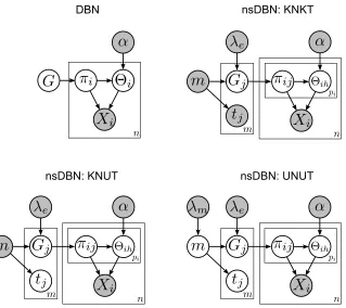
Each of the following subsections demonstrates a method for calculating an nsDBN under a variety of settings that differ in terms of the level of uncertainty about the number and times of transitions. The different settings will be abbreviated according to the type of uncertainty: whether the number of transitions is known (KN) or unknown (UN) and whether the transition times themselves are known (KT) or unknown (UT). Figure 2 shows plate diagrams relating the DBN model to the three different settings of the nsDBN model, described in the following subsections.
4.1 Known Number and Known Times of Transitions (KNKT)
In the KNKT setting, we know all of the transition times a priori; therefore, we only need to identify the most likely initial network G1and sets of edge changes∆g1, . . . ,∆gm−1. Thus, we wish
to maximize Equation (5).
To create a move set that results in an effectively mixing chain, we consider which types of local moves result in jumps between posterior modes. As mentioned earlier, networks that differ by a single edge will probably have similar likelihoods. Therefore, the move set includes a single edge addition or deletion to G1. Each of these moves results in the structural difference of a single edge over all observations. One can also consider adding or deleting an edge in a particular∆gi;
this results in the structural difference of a single edge for all observations after ti. Finally, we
consider moving an edge from one∆gi to another, which results in the structural difference of a
Figure 2: Plate diagrams relating DBNs to nsDBNs under each setting. Gray circles represent quan-tities that are known a priori while white circles represent those that are unknown. Non-stationary DBNs may have multiple networks (m, indexed by j) and multiple different parent sets for each variable (pi for variable i, indexed by h). In the KNKT setting, the
transition times tj are known a priori, but they must be estimated in the two other
set-tings. In the KNUT setting, the number of epochs m is still known, but the transition times themselves are not. Finally, in the UNUT setting, even the number of epochs is unknown; instead a truncated geometric prior is placed on m.
4.2 Known Number But Unknown Times of Transitions (KNUT)
Knowing in advance the times at which all the transitions occur, as was assumed in the previous subsection, is often unrealistic. To relax this assumption, we now assume that while m is known, the set T is not given a priori but must also be estimated. Thus, rather than maximizing Equation (5), we maximize the expression below:
P(G1,∆g1, . . . ,∆gm−1,T|D).
procedure. The complete move set for this setting includes all of the moves described previously as well as this new local shift move, listed as M6in Table 1.
As with the last setting, the number of epochs does not change; therefore, only the prior on the number of edge changes s is used.
4.3 Unknown Number and Unknown Times of Transitions (UNUT)
In the most general UNUT setting, both the transition times T and the number of transitions are unknown and must be estimated. While this is the most interesting setting, it is also the most difficult. Since the move set from the KNUT setting provides a solution to this problem when m is known, a simple approach would be to try various values of m and then determine which value of m seems optimal. However, this approach is theoretically unsatisfying and would be incredibly slow. Instead, we will further augment the move set to allow the number of transitions to change. Since both the number of edge changes s and the number of epochs m are allowed to vary, we need to incorporate both priors mentioned in Section 3.1 when evaluating the posterior.
To allow the number of epochs m to change during sampling, we introduce merge and split operations to the move set. For the merge operation, two adjacent edge sets (∆gi and∆gi+1) are combined to create a new edge set. The transition time of the new edge set is selected to be the mean of the previous locations weighted by the size of each edge set: ti′= (siti+si+1ti+1)/(si+si+1). For
the split operation, an edge set∆giis randomly chosen and randomly partitioned into two new edge
sets∆g′iand∆g′i+1with all subsequent edge sets re-indexed appropriately. Each new transition time is selected as described above. The move set is completed with the inclusion of the add transition time and delete transition time operations. These moves are similar to the split and merge operations except they also increase or decrease s, the total number of edge changes in the structure. The four additional moves are listed as M7–M10in Table 1.
4.4 MCMC Sampler Implementation Details
In practice, the sampler is designed so that the proposal ratio pp((MM′))pp((xx|′x|x′,,MM′)) is exactly 1 for most
moves. For example, if either move M1 or move M2is randomly selected, the sampling procedure is as follows: random variables xi and xjare selected, if the edge xi→xj exists in G1, it is deleted, otherwise it is added (subject to the maximum of pmaxparents constraint). We know that the
max-imal number of edges in G1 is npmax(due to the maximum parent constraint) and we let E1be the
current number of edges in G1. If we are making move M1, the probability that we select a legal edge to add is Pa =npnpmaxmax−E1. The probability of making the reverse move (from x′ back to x) is
Pd=npE1+max1. The resulting proposal ratio is thus:
Pd
Pa
p(x|x′,M2′) p(x′|x,M
1)
= E1+1 npmax−E1
npmax−E1 E1+1
=1.
A similar approach can be applied to the other moves.
This paradigm also handles boundary cases: if G1is complete, then P(M1) =0; if G1is empty, then P(M2) =0; if si=smax∀i, then P(M3) =0; if si=1∀i, then P(M4) =0; etc.
The relative proposal probabilities between different moves are designed so that all pairs of complementary moves (a move and its reverse move) are equally likely. Under the KNKT setting, Pa+Pd=Pae+Pde=2Pme. Under the KNUT setting, Pa+Pd =Pae+Pde=2Pme=2Pst. Finally,
Move type M probabilityProposal pp((MM′)) pp((xx|′x|x′,,MM′))
(M1)add edge to G1 Pa PPda
(E1+1)−1
(npmax−E1)−1= npmax−E1
E1+1
(M2)delete edge from G1 Pd PPda (npmax−E1+1) −1 E−11 =
E1 npmax−E1+1
(M3)add edge to∆gi Pae PPdeae
m−1(S
i+1)−1 m−1(Smax−Si)−1=
Smax−Si Si+1
(M4)delete edge from∆gi Pde Pae Pde
m−1(S
max−Si+1)−1 m−1S−1
i
= Si Smax−Si+1 (M5)move edge from∆gito∆gj Pme 1 (m−1)
−1(∑
iSi)−1
(m−1)−1(∑
iSi)−1= 1 (M6)locally shift ti Pst 1 (2d+1)
−1
(2d+1)−1= 1
(M7)merge∆giand∆gi+1 Pm PPms
(m−1)−12(S
i+Si+1)−1(Si+SiSi+1)
−1
(m−1)−1 = 2
(Si+Si+1)(Si+SiSi+1)
(M8)split∆gi Ps Pm Ps
(m−1)−1
(m−1)−1(Si/2)−1(Si x)
−1=(Si/2) Si
x
(M9)create new∆gi Pag Pdg Pag
(m+1)−1
(N−m)−1n−2=
(N−m)n2 m+1
(M10)delete∆gi Pdg PPagdg (N−m−1) −1n−2
m−1 =(N−mm−1)n2
K
N
K
T KN
U T U N U T 1
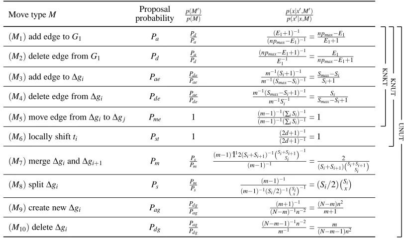
Table 1: The move sets under different settings. E1is the total number of edges in G1, pmax is the
maximum parent set size, smaxis the maximum number of edge changes allowed in a single
transition time, and siis the number of edge changes in the set∆gi. The proposal ratio is
the product of the last two columns. The KNKT setting uses moves M1–M5, KNUT uses moves M1–M6, and UNUT uses moves M1–M10, in each case with the proposal probabili-ties appropriately normalized to add to 1.
5. Results on Simulated and Real Data Sets
Here we examine both the speed and accuracy of our sampling algorithm under all three settings and on both simulated and real data sets. We want to solve real-world problems, but accurate ground truths are often not available to assess performance; therefore, we must rely on simulation studies to provide representative performance estimates for the real problems of interest.
We have studied the performance characteristics of our algorithm in simulation studies that vary by several orders of magnitude in number of observations, number of variables, number of epochs, and network density. In each case, we perform simulations with multiple data sets multiple times with multiple chains to help ensure our results are robust to simulation artifacts. For brevity, we only present a few simulation results here; the broader set of experiments we have conducted yield similar results.
All experiments were run on a 3.6GHz dual-core Intel Xeon machine with 4 GB of RAM.
5.1 Small Simulated Data Set
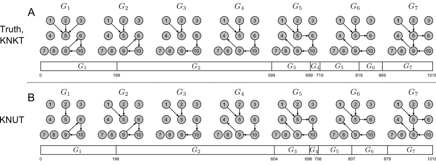
Figure 3: nsDBN structure learning with known numbers of transitions. A: True non-stationary data-generation process. The structure evolves gradually from the network at the left la-beled G1to the network at the right labeled G7. The epochs in which the various networks are active are shown in the horizontal bars, roughly to scale. The horizontal bars repre-sent the segmentation of the 1020 observations, with the transition times labeled below. When these times are known to the algorithm (the KNKT setting), the recovered nsDBN structure is exactly the true structure. B: When the times of the transitions are not known (the KNUT setting), the algorithm learns the model-averaged nsDBN structure shown (selecting edges that occur in greater than fifty percent of the sampled structures). The learned networks and most likely transition times are highly accurate (only missing two edges in G1and all predicted transition times close to the truth).
true structure is shown in Figure 3A. We chose a small network with features biologically relevant to genetic regulatory networks: a feedback loop, a variable with at least three parents, a pathway of length six, and the inclusion of observed variables that do not even participate in the network.
5.1.1 KNKT SETTING
In this simple setting, the sampler rapidly converges to the correct solution. We generate a data set using the structure in Figure 3A, and run our sampler for 100,000 iterations, with the first 25,000 samples thrown out for burn-in.
To obtain a consensus (model averaged) structure prediction, an edge is considered present at a particular time if the posterior probability of the edge is greater than 0.5. The value ofλmhas no
effect in this setting, and the value ofλs is varied between 0.1 and 50. The predicted structure is
exactly identical to the true structure shown in Figure 3A for a broad range of values, 0.5≤λs≤10,
indicating robust and accurate learning.
5.1.2 KNUT SETTING
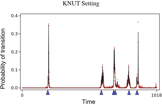
KNUT Setting
Figure 4: Posterior probability of transition times when learning an nsDBN in the KNUT setting. The blue triangles on the baseline represent the true transition times and the red dots represent one standard deviation from the mean probability, which is drawn as a black line. The variance estimates were obtained using multiple chains. The highly probable transition times correspond closely with the true transition times.
Again, we generate a data set using the structure from Figure 3A and run the sampler for 200,000 iterations, with the first 50,000 samples thrown out for burn-in. More samples are collected in the KNUT setting because we expect that convergence will be slower given the larger space of nsDBNs to explore.
The predicted consensus structure is shown in Figure 3B forλs=5; this choice ofλsprovides
the most accurate predictions. The estimated structure and transition times are very close to the truth. All edges are correct, with the exception of two missing edges in G1, and the predicted transition times are all within 10 of the true transition times. We can also examine the posterior probabilities of transition times over all sampled structures. This is shown in Figure 4. The blue triangles on the baseline represent the true transition times, and spikes represent transition times that frequently occurred in the sampled structures. While the highest probability regions do occur near the true transition times, some uncertainty exists about the exact locations of t3and t4since the fourth epoch is exceedingly short.
5.1.3 UNUT SETTING
Finally, we consider the UNUT setting where the number and times of transitions are both unknown. We examine the accuracy of our method in this setting using several values ofλsandλm. We use
the range 1≤λs≤5 because we know from the previous settings that the most accurate solutions
were obtained using a prior within this range; the range 1≤λm≤50 is selected to provide a wide
range of estimates for the prior on m since we have no previous knowledge of what it should be.
Again, we generate a data set using the structure from Figure 3A and run the sampler for 300,000 iterations, with the first 75,000 samples thrown out for burn-in. We collect samples from 25 chains in this setting.
Figure 5 shows the posterior probabilities of transition times for various settings ofλsandλm.
As expected, whenλm increases, the number of peaks decreases. Essentially, when λm is large,
only the few transition times that best characterize the non-stationary behavior of the data will be identified. On the other hand, whenλmis very small, noises within the data begin to be identified
as transition times, leading to poor estimates of transition times.
We can also examine the posterior on the number of epochs, as shown in Figure 6. The largest peak can be used to provide an estimate of m. A smallerλmresults in more predicted epochs and
less confidence about the most probable value of m.
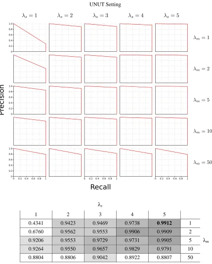
Finally, since we know what the true structure is, we can obtain a precision-recall curve for each value ofλsandλm. The precision-recall curves are shown at the top of Figure 7. To calculate these
values, we obtained individual precision and recall estimates for each network at each observation and averaged them over all observations. Therefore, the reported precision and recall values can be viewed as the average precision and average recall over all observations.
One way to identify the best parameter settings forλsandλmis to examine the best F1-measure
(the harmonic mean of the precision and recall) for each. The table in Figure 7 shows the best F1-measures and revealsλs=5 andλm=1 as best for this data, although nearly all choices achieve an
F1-measure above 0.9.
5.2 Larger Simulated Data Set
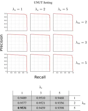
To evaluate the scalability of our technique in the most difficult UNUT setting, we also simulate data from a 100 variable network with an average of 50 edges over five epochs spanning 4800 observations, with one to three edges changing between each epoch. We generate 10 different data sets from the model and acquire 25 chains from each data set. For each chain, we take 800,000 samples, with the first 200,000 samples thrown out for burn-in.
The posterior probabilities of transition times and the number of epochs (corresponding to Fig-ures 5 and 6) for one of the simulated data sets are shown in Figure 8. The significantly sharper prediction for the posterior probabilities of transitions occurring at specific times is most likely due to having more observations and, thus, more confident estimates. The number of epochs with the highest posterior probability is five for all choices of priors, which is exactly the true number of epochs for this data set.
Additionally, the precision-recall curves and F1-measures are shown in Figure 9, revealing the
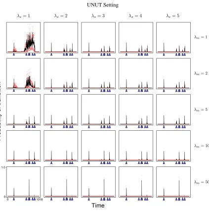
UNUT Setting
Figure 5: The posterior probabilities of transition times from the sampled structures in the UNUT setting for various values ofλsandλm. As in Figure 4, the blue triangles on the baseline
represent the true transition times and the red dots represent one standard deviation from the mean probability obtained from several runs, which is drawn as a black line. Only the (λs,λm) values of (1,1) and (1,2) seem to result in poor estimates of the true transition
times.
5.3 Drosophila Muscle Development Gene Regulatory Networks
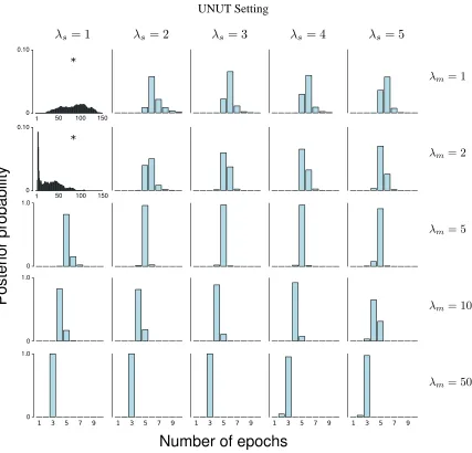
UNUT Setting
Figure 6: The posterior probabilities of the number of epochs for various values ofλsandλm. The
x-axes range from 1 to 10 and the y-axes from 0 to 1 for all of the plots except those marked with a star. The starred plots show predictions with significantly more epochs than the truth. The posterior estimates on the number of epochs m are closest to the true value of 7 whenλmis 1 or 2.
UNUT Setting
λs
1 2 3 4 5
0.4341 0.9423 0.9469 0.9738 0.9912 1
0.6760 0.9562 0.9553 0.9906 0.9909 2
0.9206 0.9553 0.9729 0.9731 0.9905 5 λm
0.9264 0.9550 0.9657 0.9829 0.9791 10
0.8804 0.8806 0.9042 0.8922 0.8807 50
Figure 7: Top: Precision-recall curves for various values ofλsandλmunder the UNUT setting. The
most accurate estimates for the structure of the nsDBN arise whenλs=5 andλm=1.
UNUT Setting
Figure 8: The posterior probabilities of transition times and number of epochs from one of the larger (100 variables, 5 epochs, and 4800 observations) simulated data sets under the UNUT setting for various values ofλsandλm. The axes are the same for all plots. Top:
UNUT Setting
λs
1 3 5
0.9489 0.9510 0.9468 1
0.9377 0.9521 0.9356 2 λm
0.9531 0.9459 0.9398 5
Figure 9: Top: Precision-recall curves for several values ofλsandλmunder the larger 100 variable
simulation. Bottom: Corresponding measures for the precision-recall curves. F1-measures over 0.9 are shaded; the highest value is shown in bold.
11 of the 19 genes identified by Zhao et al. (2006). To facilitate comparison with as many existing methods as possible, we apply our method to the data describing the expression of the same 11 genes, preprocessing the data in the same way as described by Zhao et al. (2006). Unfortunately, no other techniques predict non-stationary directed networks, so our comparisons are made against the stationary directed network predicted by Zhao et al. (2006) and the non-stationary undirected network predicted by Guo et al. (2007).
Figure 10 shows how our predicted structure compares to those reported by Zhao et al. (2006) and Guo et al. (2007). The nsDBN in Figure 10C was learned using the KNKT setting with transition times defined at the borders between the embryonic, larval, pupal, and adult stages.
While all three predictions share many edges, certain similarities between our prediction and one or both of the other two predictions are of special interest. In all three predictions, a cluster seems to form around myo61f, msp-300, up, mhc, prm, and mlc1. All of these genes except up are in the myosin family, which contains genes involved in muscle contraction. Within the directed predictions, msp-300 primarily serves as a hub gene that regulates the other myosin family genes. It is interesting to note that the undirected method predicts connections between mlc1, prm, and mhc while neither directed method makes these predictions. Since msp-300 seems to serve as a regulator to these genes, the method of Guo et al. (2007) may be unable to distinguish between direct and indirect interactions, due to its undirected nature and reliance on correlations.
Two interesting temporal similarities arise when comparing our predictions to those from Guo et al. (2007). First, an interaction between eve and actn arise at the beginning of the pupal stage in both methods. Second, the connection between msp-300 and up is lost in the adult network. Note that the loss of this edge actually characterizes the progression to the adult stage from the pupal stage in our prediction, while the method from Guo et al. (2007) combines the two stages. The estimation of a combined pupal/adult stage may simply be due to predicting the loss of the edge between msp-300 and up earlier in development than our method.
Despite the similarities, some notable differences exist between our prediction and the other two predictions. First, we predict interactions from myo61f to both prm and up, neither of which is predicted in the other methods, suggesting a greater role for myo61f during muscle development. Also, we do not predict any interactions with twi. During muscle development in Drosophila, twi acts as a regulator of mef2 which in turn regulates some myosin family genes, including mlc1 and mhc (Sandmann et al., 2006; Elgar et al., 2008); our prediction of no connection to twi mirrors this biological behavior. Finally, we note that in our predicted structure, actn never connects as a regulator (parent) to any other genes, unlike in the network predicted by Zhao et al. (2006). Since actn (actinin) only binds actin, we do not expect it to regulate other muscle development genes, even indirectly.
If we transition to the UNUT setting, we can also examine the posterior probabilities of sition times and epochs. These plots are shown in Figure 11A and 11B, respectively. The tran-sition times with high posterior probabilities correspond well to the embryonic→larval and the larval→pupal transitions, but a posterior peak occurs well before the supposed time of the pupal→adult transition; this reveals that the gene expression program governing the transition to adult morphology is active well before the fly emerges from the pupa, as would clearly be expected. Also, we see that the most probable number of epochs is three to four, mirroring closely the total number of developmental stages.
5.4 Simulated Data Set Similar to the Drosophila Data Set
Figure 10: Comparison of computationally predicted Drosophila muscle development networks. A: The directed network reported by Zhao et al. (2006). B: The undirected networks reported by Guo et al. (2007). C: The nsDBN structure learned under the KNKT setting withλs=2. Only the edges that occurred in greater than 50 percent of the samples are
shown, with thicker edges representing connections that occurred more frequently.
1 2 3 4 5 6 7 8 9 10
Time
65 0
A
B
P
rob
ab
ility
o
f t
ra
nsi
ti
on
P
oster
ior
pr
o
ba
bi
lit
y
Number of epochs
0.0 1.0
0.0 0.1 0,2 0.3 0.4
Figure 11: Learning nsDBN structure in the UNUT setting using the Drosophila muscle develop-ment data. A: Posterior probabilities of transition times usingλm=λs=2. The blue
triangles on the baseline represent the borders of embryonic, larval, pupal, and adult stages. B: Posterior probability of the number of epochs. The high weight for 3 and 4 epochs closely matches the true number of developmental stages.
Figure 12: An nsDBN was learned on simulated data that mimicked the number of nodes, connec-tivity, and transition behavior of the experimental fly data. This allowed us to estimate the accuracy of learned nsDBNs on a problem of this size. A: Precision-recall curves for increasing values of the signal to noise ratio in the data (using one replicate). B: Pre-cision recall curves for an increasing number of experimental replicates (using an SNR of 2:1). A greater signal to noise ratio and a greater number of experimental replicates both result in better performance, as expected.
As discussed earlier, to obtain posterior estimates of quantities of interest, such as the number of epochs or transition times, we generate many samples from several chains; averaging over chains provides a more efficient exploration of the sample space. To incorporate replicates into the posterior calculations, we generate samples from multiple chains (25) for each set of replicates. Since the underlying data generation process is the same for each replicate, we simply average over all the chains. The results of these simulations are summarized in Figure 12.
As expected, as the signal-to-noise ratio of the data increases, the greater the accuracy in the learned nsDBNs as reflected in the F1-measures: 1:1 is 0.734, 2:1 is 0.850, 3:1 is 0.875, and 4:1 is 0.950. Additionally, increasing the number of replicates also increases prediction accuracy: one is 0.869, two is 0.924, three is 0.945, and four is 0.956. This demonstrates the importance of multiple replicates for biological data with many variables but few observations.
5.5 Neural Information Flow Networks in Songbirds
Our goal is to learn neural information flow networks in the songbird brain. Such networks repre-sent the transmission of information between different regions of the brain. Like roads, the anatom-ical connectivity of a brain indicates potential pathways along which information can travel. Like traffic, neural information flow networks represent the dynamic utilization of these pathways. By identifying the neural information flow networks in songbirds during auditory stimuli, we hope to understand how sounds are stored and processed in the brain.
In this experiment, eight electrodes were placed into the vocal nuclei of six female zebra finches. Voltage changes were recorded from populations of neurons while the birds were provided with four different two-second auditory stimuli, each presented twenty times. The resulting voltages were post-processed with an RMS transformation and binned to 5 ms; this interval was chosen because it takes 5–10 ms for a neural signal to propagate through one synaptic connection (Kimpo et al., 2003). We analyze data recorded from electrodes for two seconds pre-stimulus, two seconds during stimulus, and two seconds post-stimulus. We learn an nsDBN for two of the birds over six seconds for two different stimuli using all repetitions; this data set contains 8 variables and nearly 25,000 observations for each bird and each stimulus.
Number of epochs Time (s) P rob ab ility o f t ra nsi ti on Song White noise Bird 1 Bird 2 Song White noise 0 0.2 0.4 0.6 0.8 1.0
0 1 2 3 4 5 6
0 0.2 0.4 0.6 0.8 1.0
0 1 2 3 4 5 6
0 0.2 0.4 0.6 0.8 1.0
0 1 2 3 4 5 6
0 0.2 0.4 0.6 0.8 1.0
0 1 2 3 4 5 6
P rob ab ility o f t ra nsi ti on Time (s) 0 1.0
1 2 3 4 5 6 0
1.0
1 2 3 4 5 6
1 2 3 4 5 6 1 2 3 4 5 6
A B
Figure 13: Posterior results of learning nsDBNs under the UNUT setting for two birds presented with two different stimuli (white noise and song). A: Posterior transition time probabili-ties. Transitions are consistently predicted near the stimulus onset (2 seconds) and offset (4 seconds). B: Posterior estimates of the number of epochs. The estimated number of epochs is three or four, with strong support for the value four when the bird is presented with a song.
The posterior transition time probabilities and the posterior number of epochs for two birds presented with two different stimuli under the UNUT setting (λs=λm=2) can be seen in Figure 13.
The posterior estimates consistently differ when the bird is listening to white noise versus song. When listening to a song, an additional transition is predicted 300–400 ms after the onset of a song but not after the onset of white noise. This implies that the bird further analyzes a sound after recognizing it (e.g., hearing a known song), but performs no further analysis when it does not recognize a sound (e.g., hearing white noise).
Previous analysis of this data assumed that any changes in the neural information flow network of a songbird listening to sound occurred only at sound onset and offset (Smith et al., 2006). Only by appropriately modeling the neural information flow networks as nsDBNs are we able to learn that this assumption is not accurate.
Further analysis and investigation of this data is left to future work.
5.6 Performance and Scalability
Due to the use of efficient data structures in the sampler implementation, the computational time needed to update the likelihood is essentially the same for all moves. Therefore, the runtimes of the algorithm under the KNKT, KNUT, and UNUT settings do not differ for a given number of samples. Nevertheless, one typically wants more samples in settings with increased uncertainty to ensure proper convergence.
For the small ten variable simulated data set, the sample collection process for each chain takes about 10 seconds per 100,000 samples, which translates to 10 seconds for the KNKT setting, 20 seconds for the KNUT setting, and 30 seconds for the UNUT setting. Fortunately, all runs can easily be executed in parallel. Sample collection for the Drosophila data set and the similarly sized simulated data set takes only a few seconds for each chain under all settings.
For the larger 100 variable simulated data set, sample collection takes about 2 minutes per 100,000 samples. The increased runtime is primarily due to the larger number of variables, so defining the neighborhood for each move takes more time. Due to intelligent caching schemes, the number of observations affects runtime in only a sublinear fashion (provided that enough memory is available).
Surprisingly, one of the largest contributors to running time is the actual recording of the MCMC samples. For example, each sample in the larger simulated data set can be represented by a 10,000 by 4,800 binary matrix of indicators for individual edges at every point in time. A full recording of each sample is therefore very time consuming: just recording each sample in the larger simulated data set leads to an increased runtime of about 50 minutes per 100,000 samples. We can alleviate this problem in several ways. First, because only a small number of those 48 million values actually change between samples, each sample can be represented and output in a compressed fashion; however, the same amount of processing still must occur after the sample collection completes. A better option is to only record the posterior quantities of interest. For example, recording just the transition times and number of epochs adds only a few seconds to the runtime on the larger simulated data set.
6. Discussion
choice of hyper-parameters over a large range of values. Additionally, by using a sampling-based approach, our method allows us to assess a confidence for each predicted edge—an advantage that neither Zhao et al. (2006) nor Guo et al. (2007) share.
We have demonstrated the feasibility of learning an nsDBN in all three settings using simulated data sets of various numbers of transition times, observations, variables, epochs, and connection densities. Additionally, we have identified nsDBNs in the KNKT and UNUT settings using biologi-cal gene expression data. The Drosophila muscle development network we predict is consistent with the predictions from other techniques and conforms to many known biological interactions from the literature. The predicted transition times and number of epochs also correspond to the known times of large developmental changes. Although each connection on the predicted Drosophila muscle de-velopment network is difficult to verify, simulated experiments of a similar scale demonstrate highly accurate predictions, even with moderately noisy data and one replicate.
While we focus on certain aspects of the model in this paper, many of our decisions are choices rather than restrictions. For example, we present results using a Markov lag of one, but any Markov lag could be used. Additionally, we use the BDe score metric, but any score metric or conditional independence test can be used instead; however, any score metric which does not integrate over the non-structural parameters would require an augmented sampling procedure. The assumption of discrete data is not necessary; our method easily extends to continuous data, provided that an appropriate scoring metric (like BG) is adapted.
A discrete view of time is necessary to our approach, but many continuous-time data sets can be transformed into discrete-time ones without significant loss of information. The use of directed graphs is also necessary, and desired, but undirected estimates can be obtained through moralization of directed estimates. Although we choose simple priors to learn smoothly evolving networks, nearly any priors would be easy to incorporate; in particular, incorporating expert knowledge about the problem domain would be an ideal method for defining priors.
For problems of more than a few variables, the use of MCMC sampling is essential since EM techniques would not converge in any reasonable time frame given such a large sample space. One of our key discoveries for increasing convergence is the reformulation of the problem from learning multiple networks to learning a network and changes to that network. This parameterization pro-vides an intuitive means for defining evolving networks and allows us to define move sets with good convergence properties. Our particular choices of the move sets are not the only possible ones, but we have taken extra care to ensure that they work well on the types of problems we examine in this paper.