Efficient Heuristics for Discriminative Structure Learning of Bayesian
Network Classifiers
Franz Pernkopf [email protected]
Department of Electrical Engineering Graz University of Technology A-8010 Graz, Austria
Jeff A. Bilmes [email protected]
Department of Electrical Engineering University of Washington
Seattle, WA 98195, USA
Editor: Russ Greiner
Abstract
We introduce a simple order-based greedy heuristic for learning discriminative structure within generative Bayesian network classifiers. We propose two methods for establishing an order of N features. They are based on the conditional mutual information and classification rate (i.e., risk), respectively. Given an ordering, we can find a discriminative structure withO Nk+1
score evalu-ations (where constant k is the tree-width of the sub-graph over the attributes). We present results on 25 data sets from the UCI repository, for phonetic classification using the TIMIT database, for a visual surface inspection task, and for two handwritten digit recognition tasks. We provide classification performance forbothdiscriminativeandgenerative parameter learning onboth dis-criminativelyandgeneratively structured networks. The discriminative structure found by our new procedures significantly outperforms generatively produced structures, and achieves a classifica-tion accuracy on par with the best discriminative (greedy) Bayesian network learning approach, but does so with a factor of∼10-40 speedup. We also show that the advantages of generative discrim-inatively structured Bayesian network classifiers still hold in the case of missing features, a case where generative classifiers have an advantage over discriminative classifiers.
Keywords: Bayesian networks, classification, discriminative learning, structure learning,
graphi-cal model, missing feature
1. Introduction
Bayesian networks (Pearl, 1988; Cowell et al., 1999) have been widely used as a space within which to search for high performing statistical pattern classifiers. Such networks can be produced in a number of ways, and ideally the structure of such networks will be learned discriminatively. By “discriminative learning” of Bayesian network structure, we mean simply that the process of learn-ing corresponds to optimizlearn-ing an objective function that is highly representative of classification error, such as maximizing class conditional likelihood, or minimizing classification error under the 0/1-loss function or some smooth convex upper-bound surrogate (Bartlett et al., 2006).
that learning paths (Meek, 1995), polytrees (Dasgupta, 1997), k-trees (Arnborg et al., 1987) or bounded tree-width graphs (Karger and Srebro, 2001; Srebro, 2003), and general Bayesian networks (Geiger and Heckerman, 1996) are all instances of NP-complete optimization problems. Learning the best “discriminative structure” is no less difficult, largely because the cost functions that are needed to be optimized do not in general decompose (Lauritzen, 1996), but there has as of yet not been any formal hardness results in the discriminative case.
Discriminative optimization of a Bayesian network structure for the purposes of classification does have its advantages, however. For example, the resulting networks are amenable to interpre-tation compared to a purely discriminative model (the structure specifies conditional independen-cies between variables that may indicate distinctive aspects of how best to discern between objects Bilmes et al., 2001), it is simple to work with missing features and latent variables (as we show in this paper), and to incorporate prior knowledge (see below for further details). Since discrimi-native learning of such networks optimizes for only one inference scenario (e.g., classification) the resulting networks might be simpler or more parsimonious than generatively derived networks, may better abide Occam’s razor, and may restore some of the benefits mentioned in Vapnik (1998).
Many heuristic methods have been produced in the past to learn the structure of Bayesian net-work classifiers. For example, Friedman et al. (1997) introduced the tree-augmented naive (TAN) Bayes approach, where a naive Bayes (NB) classifier is augmented with edges according to various
conditional mutual information criteria. Bilmes (1999, 2000) introduced theexplaining away
resid-ual (EAR) for discriminative structure learning of dynamic Bayesian networks for speech recogni-tion applicarecogni-tions, which also happens to correspond to “synergy” in the neural code (Brenner et al., 2000). The EAR measure is in fact an approximation to the expected class conditional distribution, and so improving EAR is likely to decrease the KL-divergence between the true class posterior and the resultant approximate class posterior. A procedure for providing a local optimum of the EAR measure was outlined in Narasimhan and Bilmes (2005) but it may be computationally expensive. Greiner and Zhou (2002); Greiner et al. (2005) express general Bayesian networks as standard lo-gistic regression—they optimize parameters with respect to the conditional likelihood (CL) using a conjugate gradient method. Similarly, Roos et al. (2005) provide conditions for general Bayesian networks under which the correspondence to logistic regression holds. In Grossman and Domin-gos (2004) the conditional log likelihood (CLL) function is used to learn a discriminative structure. The parameters are set using maximum likelihood (ML) learning. They use a greedy hill climbing search with the CLL function as a scoring measure, where at each iteration one edge is added to the structure which conforms with the restrictions of the network topology (e.g., TAN) and the
acyclic-ity property of Bayesian networks. In a similar algorithm, the classification rate (CR)1 has also
been used for discriminative structure learning (Keogh and Pazzani, 1999; Pernkopf, 2005). The hill climbing search is terminated when there is no edge which further improves the CR. The CR is the discriminative criterion with the fewest approximations, so it is expected to perform well given sufficient data. The problem, however, is that this approach is extremely computationally expensive, as a complete re-evaluation of the training set is needed for each considered edge. Many generative structure learning algorithms have been proposed and are reviewed in Heckerman (1995), Murphy (2002), Jordan (1999) and Cooper and Herskovits (1992). Independence tests may also be used for generative structure learning using, say, mutual information (de Campos, 2006) while other recent
independence test work includes Gretton and G¨yorfi (2008) and Zhang et al. (2009). An experimen-tal comparison of discriminative and generative parameter training on both discriminatively and generatively structured Bayesian network classifiers has been performed in Pernkopf and Bilmes (2005). An empirical and theoretical comparison of certain discriminative and generative classifiers (specifically logistic regression and NB) is given in Ng and Jordan (2002). It is shown that for small sample sizes the generative NB classifier can outperform the discriminative model.
This work contains the following offerings. First, a new case is made for why and when dis-criminatively structured generative models can be usefully used to solve multi-class classification problems.
Second, we introduce a new order-based greedy search heuristic for finding discriminative struc-tures in generative Bayesian network classifiers that is computationally efficient and that matches the performance of the currently top-performing but computationally expensive greedy “classifi-cation rate” approach. Our resulting classifiers are restricted to TAN 1-tree and TAN 2-trees, and so our method is a form of search within a complexity-constrained model space. The approach we employ looks first for an ordering of the N features according to classification based informa-tion measures. Given the resulting ordering, the algorithm efficiently discovers high-performing
discriminative network structure with no more than
O
Nk+1score evaluations where k indicates the tree-width of the sub-graph over the attributes, and where a score evaluation can either be a mutual-information or a classification error-rate query. Our order-based structure learning is based on the observations in Buntine (1991) and the framework is similar to the K2 algorithm proposed in Cooper and Herskovits (1992). We use, however, a discriminative scoring metric and suggest approaches for establishing the variable ordering based on conditional mutual information (CMI) (Cover and Thomas, 1991) and CR.
Lastly, we provide a wide variety of empirical results on a diverse collection of data sets showing that the orderbased heuristic provides comparable classification results to the best procedure -the greedy heuristic using -the CR score, but our approach is computationally much cheaper. Fur-thermore, we empirically show that the chosen approaches for ordering the variables improve the classification performance compared to simple random orderings. We experimentally compare both discriminative and generative parameter training on both discriminative and generatively structured Bayesian network classifiers. Moreover, one of the key advantages of generative models over dis-criminative ones is that it is still possible to marginalize away any missing features. If it is not known at training time which features might be missing, a typical discriminative model is rendered unusable. We provide empirical results showing that discriminatively learned generative models are reasonably insensitive to such missing features and retain their advantages over generative models in such case.
et al., 1998) and USPS data set. Last, Section 7 concludes. We note that a preliminary version of a subset of our results appeared in Pernkopf and Bilmes (2008b).
2. Bayesian Network Classifiers
A Bayesian network (BN) (Pearl, 1988; Cowell et al., 1999)
B
=hG
,Θiis a directed acyclic graphG
= (Z,E)consisting of a set of nodes Z and a set of directed edges E=EZi,Zj,EZi,Zk, . . . con-necting the nodes where EZi,Zj is an edge directed from Zito Zj. This graph represents factorization properties of the distribution of a set of random variables Z={Z1, . . . ,ZN+1}. Each variable in
Z has values denoted by lower case letters{z1,z2, . . . ,zN+1}. We use boldface capital letters, for
example, Z, to denote a set of random variables and correspondingly boldface lower case letters denote a set of instantiations (values). Without loss of generality, in Bayesian network classifiers the random variable Z1represents the class variable C∈ {1, . . . ,|C|},|C|is the cardinality of C or
equivalently the number of classes, X1:N={X1, . . . ,XN}={Z2, . . . ,ZN+1}denote the set of random
variables of the N attributes of the classifier. Each graph node represents a random variable, while the lack of edges in a graph specifies some conditional independence relationships. Specifically, in a Bayesian network each node is independent of its non-descendants given its parents (Lauritzen, 1996). A Bayesian network’s conditional independence relationships arise due to missing parents in the graph. Moreover, conditional independence can reduce computation for exact inference on
such a graph. The set of parameters which quantify the network are represented byΘ. Each node
Zjis represented as a local conditional probability distribution given its parents ZΠj. We useθ j i|hto denote a specific conditional probability table entry (assuming discrete variables), the probability that variable Zj takes on its ith value assignment given that its parents ZΠj take their h
th
(lexico-graphically ordered) assignment, that is,θij|h=PΘ Zj=i|ZΠj =h
. Hence, h contains the parent configuration assuming that the first element of h, that is, h1, relates to the conditioning class and
the remaining elements h\h1denote the conditioning on parent attribute values. The training data
consists of M independent and identically distributed samples
S
={zm}Mm=1 =
cm,xm1:N Mm=1. For most of this work, we assume a complete data set with no missing values (the exception being Section 6.6 where input features are missing at test time). The joint probability distribution of the network is determined by the local conditional probability distributions as
PΘ(Z) = N+1
∏
j=1
PΘ Zj|ZΠj
and the probability of a sample zmis
PΘ(Z=zm) = N+1
∏
j=1
|Zj|
∏
i=1
∏
hθj i|h
uij|,hm
,
where we introduced an indicator function uij|,hmof the mthsample
uij|,hm=
1, if zmj =i and zmΠ
j =h
0, otherwise .
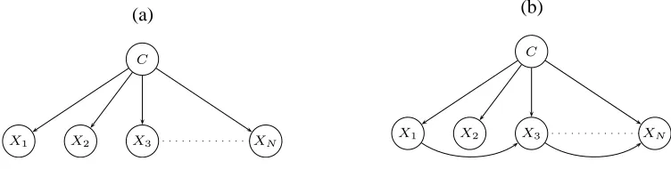
all the attributes are conditionally independent given the class label. This means that, given C, any subset of X is independent of any other disjoint subset of X. As reported in the literature (Friedman et al., 1997; Domingos and Pazzani, 1997), the performance of the NB classifier is surprisingly good even if the conditional independence assumption between attributes is unrealistic or even false in most of the data. Reasons for the utility of the NB classifier range between benefits from the bias/variance tradeoff perspective (Friedman et al., 1997) to structures that are inherently poor from a generative perspective but good from a discriminative perspective (Bilmes, 2000). The structure of the naive Bayes classifier represented as a Bayesian network is illustrated in Figure 1a.
(a)
C
X1 X2 X3 XN
(b)
C
X1 X2 X3 XN
Figure 1: Bayesian Network: (a) NB, (b) TAN.
In order to correct some of the limitations of the NB classifier, Friedman et al. (1997) intro-duced the TAN classifier. A TAN is based on structural augmentations of the NB network, where additional edges are added between attributes in order to relax some of the most flagrant conditional independence properties of NB. Each attribute may have at most one other attribute as an additional parent which means that the tree-width of the attribute induced sub-graph is unity, that is, we have to learn a 1-tree over the attributes. The maximum number of edges added to relax the independence
assumption between the attributes is N−1. Thus, two attributes might not be conditionally
inde-pendent given the class label in a TAN. An example of a TAN 1-tree network is shown in Figure 1b. A TAN network is typically initialized as a NB network and additional edges between attributes are determined through structure learning. An extension of the TAN network is to use a k-tree, that is, each attribute can have a maximum of k attribute nodes as parents. In this work, TAN and k-tree
structures are restricted such that the class node remains parent-less, that is, CΠ=/0. While many
other network topologies have been suggested in the past (and a good overview is provided in Acid et al., 2005), in this work we keep the class variable parent-less since it allows us to achieve one of our goals, which is to concentrating on generative models and their structures.
3. Discriminative Learning in Generative Models
desirable because they are amenable to interpretation (e.g., the structure of a generative Bayesian network specifies conditional independencies between variables that might have a useful high-level explanation). Additionally, they are amenable to a variety of probabilistic inference scenarios ow-ing to the fact that they often decompose (Lauritzen, 1996)—the decomposition (or factorization) properties of a model are often crucial to their efficient computation.
Discriminative approaches, on the other hand, more directly represent aspects of the distribution that are important for classification accuracy, and there are a number of ways this can be done. For example, some approaches model only the class posterior probability (the conditional probability
of the class given the features) or p(C|X). Other approaches, such as support vector machines
(SVMs) (Sch¨olkopf and Smola, 2001; Burges, 1998) or neural networks (Bishop, 2006, 1995), directly model information about decision boundary sometimes without needing to concentrate on obtaining an accurate conditional distribution (neural networks, however, are also used to produce conditional distributions above and beyond just getting the class ranks correct Bishop, 1995). In each case, the objective function that is optimized is one whose minima occur not necessarily when the joint distribution p(C,X)is accurate, but rather when the classification error rate on a training set is small. Discriminative models are usually restricted to one particular inference scenario, that is, the mapping from observed input features X to the unknown class output variable C, and not the other way around.
There are several reasons for using discriminative rather than generative classifiers, one of which is that the classification problem should be solved most simply and directly, and never via a more general problem such as the intermediate step of estimating the joint distribution (Vapnik, 1998). The superior performance of discriminative classifiers has been reported in many application do-mains (Ng and Jordan, 2002; Raina et al., 2004; Juang et al., 1997; Juang and Katagiri, 1992; Bahl et al., 1986).
Why then should we have an interest in generative models for discrimination? We address this question in the next several paragraphs. The distinction between generative and discriminative mod-els becomes somewhat blurred when one considers that there are both generative and discriminative methods to learn a generative model, and within a generative model one may make a distinction between learning model structure and learning its parameters. In fact, in this paper, we make a clear distinction between learning the parameters of a generative model and learning the structure of a generative model. When using Bayesian networks to describe factorization properties of generative models, the structure of the model corresponds to the graph: fixing the graph, the parameters of the model are such that they must respect the factorization properties expressed by that graph. The structure of the model, however, can be independently learned, and different structures correspond to different families of graph (each family is spanned by the parameters respecting a particular structure). A given structure is then evaluated under a particular “best” set of parameter values, one possibility being the maximum likelihood settings. Of course, one could consider optimizing both parameters and structure simultaneously. Indeed, both structure and parameters are “parameters” of the model, and it is possible to learn the structure along with the parameters when a complexity
penalty is applied that encourages sparse solutions, such asℓ1-regularization (Tibshirani, 1996) in
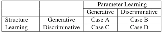
Moreover, both parameters and structure of a generative model can be learned either genera-tively or discriminagenera-tively. Discriminative parameter learning of generative models, such as hidden Markov models (HMMs) has occurred for many years in the speech recognition community (Bahl et al., 1986; Ephraim et al., 1989; Ephraim and Rabiner, 1990; Juang and Katagiri, 1992; Juang et al., 1997; Heigold et al., 2008), and more recently in the machine learning community (Greiner and Zhou, 2002; Greiner et al., 2005; Roos et al., 2005; Ng and Jordan, 2002; Bishop and Lasserre, 2007; Pernkopf and Wohlmayr, 2009). Discriminative structure learning has also more recently re-ceived some attention (Bilmes, 1999, 2000; Pernkopf and Bilmes, 2005; Keogh and Pazzani, 1999; Grossman and Domingos, 2004). In fact, there are four possible cases of learning a generative model as depicted in Figure 2. Case A is when both structure and parameter learning is generative. Case B is when the structure is learned generatively, but the parameters are learned discriminatively. Case C is the mirror image of case B. Case D, potentially the most preferable case for classification, is where both the structure and parameters are discriminatively learned.
Parameter Learning
Generative Discriminative
Structure Learning
Generative Case A Case B
Discriminative Case C Case D
Figure 2: Learning generative-model based classifiers: Cases for each possible combination of gen-erative and discriminative learning of either the parameters or the structure of Bayesian network classifiers.
In this paper, we are particularly interested in learning the discriminative structure of a gener-ative model. With a genergener-ative model, even discrimingener-atively structured, some aspect of the joint distribution p(C,X)is still being represented. Of course, a discriminatively structured generative model needs only represent that aspect of the joint distribution that is beneficial from a classifica-tion error rate perspective, and need not “generate” well (Bilmes et al., 2001). For this reason, it is likely that a discriminatively trained generative model will not need to be as complex as an accurate generatively trained model. In other words, the advantage of parsimony of a discriminative model over a generative model will likely be partially if not mostly recovered when one trains a generative model discriminatively. Moreover, there are a number of reasons why one might, in certain contexts, prefer a generative to a discriminative model including: parameter tying and domain knowledge-based hierarchical decomposition is facilitated; it is easy to work with structured data; there is less sensitivity to training data class skew; generative models can still be trained and structured discrim-inatively (as mentioned above); and it is easy to work with missing features by marginalizing over the unknown variables. This last point is particularly important: a discriminatively structured gen-erative model still has the ability to go from p(C,X)to p(C,X′)where X′is a subset of the features in X. This amounts to performing the marginalization p(C,X′) =∑X\X′p(C,X), something that
Learning a discriminatively structured generative model is inherently a combinatorial optimiza-tion problem on a “discriminative” objective funcoptimiza-tion. This means that there is an algorithm that operates by tending to prefer structures that perform better on some measure that is related to clas-sification error. Assuming sufficient training data, the ideal objective function is empirical risk under the 0/1-loss (what we call CR, or the average error rate over training data), which can be im-plicitly regularized by constraining the optimization process to consider only a limited complexity model family (e.g., k-trees for fixed k). In the case of discriminative parameter learning, CR can be used, but typically alternative continuous and differentiable cost functions, which may upper-bound CR and might be convex (Bartlett et al., 2006), are used and include conditional (log) likelihood
CLL(
B
|S
) =log∏mM=1PΘ C=cm|X1:N =xm1:N
—this last objective function in fact corresponds to maximizing the mutual information between the class variable and the features (Bilmes, 2000), and can easily be augmented by a regularization term as well.
One may ask, given discriminative parameter learning, is discriminative structure still neces-sary? In the following, we present a simple synthetic example (similar to Narasimhan and Bilmes, 2005) and actual training and test results that indicate when a discriminative structure would be necessary for good classification performance in a generative model. The model consists of 3 bi-nary valued attributes X1,X2,X3and a binary uniformly distributed class variable C. ¯X1denotes the
negation of X1. For both classes, X1is uniformly distributed and X2=X1with probability 0.5 and a
uniformly distributed random number with probability 0.5. So we have the following probabilities for both classes:
X1:=
0 with probability 0.5
1 with probability 0.5
X2:=
X1 with probability 0.5
0 with probability 0.25
1 with probability 0.25
For class 1, X3is determined according to the following:
X3:=
X1 with probability 0.3 X2 with probability 0.5
0 with probability 0.1
1 with probability 0.1
.
For class 2, X3is given by:
X3:=
¯
X1 with probability 0.3 X2 with probability 0.5
0 with probability 0.1
1 with probability 0.1
.
For both classes, the dependence between X1−X2is strong. The dependence X2−X3is stronger
than X1−X3, but only from a generative perspective (i.e., I(X2; X3)>I(X1; X3)and I(X2; X3|C)> I(X1; X3|C)). Hence, if we were to use the strength of mutual information, or conditional mutual
information, to choose the edge, we would choose X2−X3. However, it is the X1−X3dependency
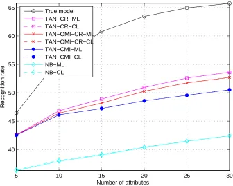
on these structures using either ML or CL (Greiner et al., 2005). For learning a generative TAN structure, we use the algorithm proposed by Friedman et al. (1997) which is based on optimizing the CMI between attributes given the class variable. For learning a discriminative structure, we apply our order-based algorithm proposed in Section 5 (we note that optimizing the EAR measure (Pernkopf and Bilmes, 2005) leads to similar results in this case).
100 200 300 400 500 600 700 800 900 1000
48 50 52 54 56 58 60 62 64 66
Sample size
Recognition rate
TAN−Discriminative Structure−ML TAN−Discriminative Structure−CL SVM
TAN−Generative Structure−ML TAN−Generative Structure−CL NB−ML
NB−CL
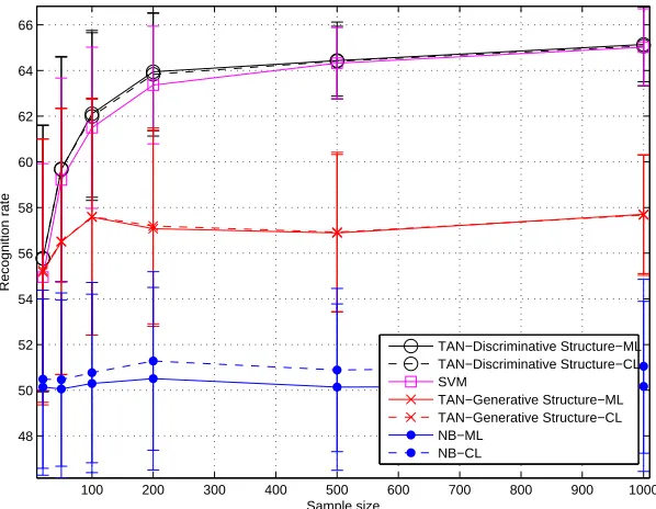
Figure 3: Generative and discriminative learning of Bayesian network classifiers on synthetic data.
Figure 3 compares the classification performance of these various cases, and in addition we show results for a NB classifier, which resorts to random guessing between both classes due to the lack of any feature dependency. Additionally, we provide the classification performance achieved
with SVMs using a radial basis function (RBF) kernel.2 On the x-axis, the training set sample size
varies according to{20,50,100,200,500,1000}and the test data set contains 1000 samples. Plots are averaged over 100 independent simulations. The solid line is the performance of the classifiers using ML parameter learning, whereas, the dashed line corresponds to CL parameter training.
(a)
X1 X2 X3
(b)
X1 X3 X2
Figure 4: (a) Generatively learned 1-tree, (b) Discriminatively learned 1-tree.
Figure 4 shows (a) the generative (b) the discriminative 1-tree over the attributes of the resulting TAN network (the class variable which is the parent of each feature is not shown in this figure).
A generative model prefers edges between X1−X2and X2−X3 which do not help discrimination.
The dependency between X1 and X3 enables discrimination to occur. Note that for this example
the difference between ML and CL parameter learning is insignificant and for the generative model, only a discriminative structure enables correct classification. The performance of the non-generative SVM is similar to our discriminatively structured Bayesian network classifier. Therefore, when a generative model is desirable (see the reasons why this might be the case above), there is clearly a need for good discriminative structure learning.
In this paper, we show that the loss of a “generative meaning” of a generative model (when it is structured discriminatively) does not impair the generative model’s ability to easily deal with missing features (Figure 11).
4. Learning Bayesian Networks
In the following sections, we briefly summarize state-of-the-art generative and discriminative struc-ture and parameter learning procedures that are used to compare our order-based discriminative structure learning heuristics (which will be described in Section 5 and evaluated in Section 6).
4.1 Generative Parameter Learning
The parameters of the generative model are learned by maximizing the log likelihood of the data which leads to the ML estimation ofθij|h. The log likelihood function of a fixed structure of
B
isLL(
B
|S
) = M∑
m=1
log PΘ(Z=zm) = M
∑
m=1
N+1
∑
j=1
log PΘ
Zj=zmj|ZΠj =z m Πj
=
M
∑
m=1
N+1
∑
j=1
|Zj|
∑
i=1
∑
huij|,hmlog
θj i|h
.
(1)
It is easy to show that the ML estimate of the parameters is
θj i|h=
∑M m=1u
j,m i|h
∑M m=1∑
|Zj| l=1u
j,m l|h
,
using Lagrange multipliers to constrain the parameters to a valid normalized probability distribution. Since we are optimizing over constrained BN structures (k-trees), we do not perform any further regularization during training other than simple smoothing to remove zero-probability entries (see Section 6.1).
4.2 Discriminative Parameter Learning
is
CLL(
B
|S
) =log M∏
m=1
PΘ(C=cm|X1:N=xm1:N) = M
∑
m=1
log PΘ C=c
m,X
1:N=xm1:N
|C|
∑
c=1
PΘ C=c,X1:N=xm1:N
=
M
∑
m=1
"
log PΘ(C=cm,X1:N =xm1:N)−log
|C|
∑
c=1
PΘ(C=c,X1:N=xm1:N)
#
.
Similar to Greiner and Zhou (2002) we use a conjugate gradient algorithm with line-search (Press
et al., 1992). In particular, thePolak-Ribiere method is used (Bishop, 1995). The derivative of the
objective function is
∂CLL(
B
|S
)∂θj i|h
= M
∑
m=1
"
∂ ∂θj
i|h
log PΘ(C=cm,X1:N=xm1:N)−
1 |C|
∑
c=1
PΘ C=c,X1:N =xm1:N
∂ ∂θj i|h
|C|
∑
c=1
PΘ(C=c,X1:N=xm1:N) #
.
Further, we distinguish two cases for deriving ∂CLL(B|S)
∂θj i|h
. For TAN, NB, or 2-tree structures each
parameter θij|h involves the class node value, either C=i for j=1 (Case A) or C=h1 for j>1
(Case B) where h1denotes the class instantiation h1∈h.
4.2.1 CASEA
For the class variable, that is, j=1 and h=/0, we get
∂CLL(
B
|S
)∂θ1
i =
M
∑
m=1
"
u1i,m
θ1 i −W m i θ1 i # ,
where we use Equation 1 for deriving the first term (omitting the sum over j and h) and we intro-duced the posterior
Wim=PΘ(C=i|X1:N =xm1:N) =
PΘ C=i,X1:N =xm1:N
|C|
∑
c=1
PΘ C=c,X1:N=xm1:N .
4.2.2 CASEB
For the attribute variables, that is, j>1, we derive correspondingly and have
∂CLL(
B
|S
)∂θj i|h
= M
∑
m=1
"
uij|,hm
θj i|h
−Whm1v
j,m i|h\h1 θj
i|h #
,
where Whm1 =PΘ C=h1|X1:N =xm1:N
is the posterior for class h1and sample m, and vij|,hm\h
1 =
1, if zmj =i and zmΠj=h\h1
The probabilityθij|h is constrained toθij|h≥0 and∑|Zj| i=1θ
j
i|h=1. We re-parameterize the problem
to incorporate the constraints of θij|h in the conjugate gradient algorithm. Thus, we use different
parametersβij|has follows
θj i|h=
exp
βj i|h
∑|Zj| l=1exp
βj l|h
.
This requires the gradient ∂CLL(B|S)
∂βj i|h
which is computed after some modifications as
∂CLL(
B
|S
)∂βj i|h
=
|Zj|
∑
k=1
∂CLL(
B
|S
)∂θj k|h
∂θj k|h
∂βj i|h
= M
∑
m=1
h
u1i,m−Wim
i
−θ1i
M
∑
m=1
|C|
∑
c=1
u1c,m−Wcm
for Case A and similarly for Case B we get the gradient
∂CLL(
B
|S
)∂βj i|h
= M
∑
m=1
h
uij|,hm−Whm1vij|,hm\h
1
i
−θij|h
M
∑
m=1
|Zj|
∑
l=1
h
ulj|,hm−Whm1vlj|,hm\h
1
i
.
4.3 Generative Structure Learning
The conditional mutual information between the attributes given the class variable is computed as:
I(Xi; Xj|C) =EP(Xi,Xj,C)log
P(Xi,Xj|C)
P(Xi|C)P(Xj|C)
.
This measures the information between Xi and Xj in the context of C. Friedman et al. (1997) gives
an algorithm for constructing a TAN network using this measure. This algorithm is an extension of the approach in Chow and Liu (1968). We briefly review this algorithm in the following:
1. Compute the pairwise CMI I(Xi; Xj|C) ∀ 1≤i≤N and i< j≤N.
2. Build an undirected 1-tree using the maximal weighted spanning tree algorithm (Kruskal, 1956) where each edge connecting Xiand Xj is weighted by I(Xi; Xj|C).
3. Transform the undirected 1-tree to a directed tree. That is, select a root variable and direct all edges away from this root. Add to this tree the class node C and the edges from C to all attributes X1, . . . ,XN.
4.4 Discriminative Structure Learning
As a baseline discriminative structure learning method, we use a greedy edge augmentation method
and also theSuperParent algorithm (Keogh and Pazzani, 1999).
4.4.1 GREEDYHEURISTICS
each iteration we add the edge that, while maintaining a partial 1-tree, gives the largest improve-ment of the scoring function (defined below). This process is terminated when there is no edge which further improves the score. This process might thus result in a partial 1-tree (forest) over the attributes. This approach is computationally expensive since each time an edge is added, the scores
for all
O
N2 edges need to be re-evaluated due to the discriminative non-decomposable scoringfunctions we employ. This method overall has cost
O
N3score evaluations to produce a 1-tree,which in the case of an
O
(NM)) score evaluation cost (such as the below), has an overall complexityof
O
N4. There are two score functions we consider: the CR (Keogh and Pazzani, 1999; Pernkopf,2005)
CR(
BS
|S
) = 1M
M
∑
m=1
δ(
BS
(xm1:N),cm) and the CL (Grossman and Domingos, 2004)CL(
B
|S
) = M∏
m=1
PΘ(C=cm|X1:N=xm1:N),
where the expressionδ
BS
xm1:N,cm=1 if the Bayesian network classifier BS xm1:N
trained with samples in
S
assigns the correct class label cmto the attribute values xm1:N, and is equal to 0other-wise.3 In our experiments, we consider the CR score which is directly related to the empirical risk
in Vapnik (1998). The CR is the discriminative criterion that, given sufficient training data, most directly judges what we wish to optimize (error rate), while an alternative would be to use a convex upper-bound on the 0/1-loss function (Bartlett et al., 2006). Like in the generative case above, since we are optimizing over a constrained model space (k-trees), and are performing simple parameter smoothing, again regularization is implicit. This approach has in the literature been shown to be the algorithm that produces the best performing discriminative structure (Keogh and Pazzani, 1999; Pernkopf, 2005) but at the cost of a very expensive optimization procedure. To accelerate this algo-rithm in our implementation of this procedure (which we use as a baseline to compare against our still to-be-defined proposed approach), we apply two techniques:
1. The data samples are reordered during structure learning so that misclassified samples from previous evaluations are classified first. The classification is terminated as soon as the perfor-mance drops below the currently best network score (Pazzani, 1996).
2. During structure learning the parameters are set to the ML values. When learning the structure
we only have to update the parameters of those nodes where the set of parents ZΠj changes.
This observation can be also used for computing the joint probability during classification. We can memorize the joint probability and exchange only the probabilities of those nodes where the set of parents changed to get the new joint probability (Keogh and Pazzani, 1999).
In the experiments this greedy heuristic is labeled as TAN-CR and 2-tree-CR for 1-tree and 2-tree structures, respectively.
4.4.2 SUPERPARENT AND ITSk-TREEGENERALIZATION
Keogh and Pazzani (1999) introduced theSuperParent algorithm to efficiently learn a discriminative
TAN structure. The algorithm starts with a NB network and the edges pointing from the class
variable to each attribute remain fixed throughout the algorithm. In the first step, each attribute in turn is considered as a parent of all other parentless attributes (except the class variable). If there are no parentless attributes left, the algorithm terminates. The parent which improves the CR the most is selected and designated the current superparent. The second step fixes the most recently chosen superparent and keeps only the single best child attribute of that superparent. The single edge between superparent and best child is then kept and the process of selecting a new superparent is repeated, unless no improvement is found at which point the algorithm terminates. The number of
CR evaluations therefore in a complete run of the algorithm is
O
N2. Moreover, CR determinationcan be accelerated as mentioned above.
We can extend this heuristic to learn 2-trees by simply modifying the first step accordingly: consider each attribute as an additional parent of all parentless or single-parented attributes (while
ensuring acyclicity), and choose as the superparent the one that evaluates best, requiring
O
(N)CR evaluations. Next, we retain the pair of edges between superparent and (parentless or
single-parented) children that evaluates best using CR, requiring
O
N2 CR evaluations. The processrepeats if successful and otherwise terminates. The obvious k-tree generalization modifies the first step to choose an additional parent of all attributes with fewer than k parents, and then selects the
best children for edge retention, leading overall to a process with
O
Nk+1score evaluations. Inthis paper, we compare against this heuristic in the case of k=1 and k=2, abbreviating them,
respectively, as TAN-SuperParent and 2-tree-SuperParent.
5. New Heuristics: Order-based Greedy Algorithms
It was first noticed in Buntine (1991); Cooper and Herskovits (1992) that the best network
consis-tent with a given variable ordering can be found with
O
(Nq+c) score evaluations where q is themaximum number of parents per node in a Bayesian network, and where c is a small fixed constant. These facts were recently exploited in Teyssier and Koller (2005) where generative structures were learned. Here, we are inspired by these ideas and apply them to the case of learning discriminative structures. Also, unlike Teyssier and Koller (2005), we establish only one ordering, and since our scoring cost is discriminative, it does not decompose and the learned discriminative structure is not guaranteed to be optimal. However, experiments show good results at relatively low computational learning costs.
Our procedure looks first for a total ordering≺of the variables X1:Naccording to certain criteria
which are outlined below. The parents of each node are chosen in such a way that the ordering is respected, and that the procedure results in at most a k-tree. We note here, a k-tree is typically defined on an undirected graphical model as one that has a tree-width of k—equivalently, there exists an elimination order in the graph such that at each elimination step, the node being eliminated has no more than k neighbors at the time of elimination. When we speak of a Bayesian network being a k-tree, what we really mean is that the moralized version of the Bayesian network is a k-tree. As a reminder, our approach is to learn a k-tree (i.e., a computationally and parameter constrained
Bayesian network) over the features X1:N. We still assume, as is done with a naive Bayes model,
that C is a parent of each Xi and this additional is not counted in k—thus, a 1-tree would have two
5.1 Step 1: Establishing an Order≺
We propose three separate heuristics for establishing an ordering≺of the attribute nodes prior to
parent selection. In each case as we will see later, we use the resulting ordering such that later features may only have earlier features as parents—this limit placed on the set of parents leads to reduced computational complexity. Two of the heuristics are based on the conditional mutual
infor-mation I(C; XA|XB) between the class variable C and some subset of the features XA given some
disjoint subset of variables XB(so A∩B=/0). The conditional mutual information (CMI) measures
the degree of dependence between the class variable and XA given XB and it may be expressed
entirely in terms of entropy via I(C; XA|XB) =−H(C,XA,XB) +H(XA,XB) +H(C,XB)−H(XB), where entropy of X is defined as H(X) =−∑xp(x)log p(x). When B= /0, we of course obtain (unconditional) mutual information. A structure that maximizes the mutual information between C and X is one that will lead to the best approximation of the posterior probability. In other words, an ideal form of optimization would do the following:
B
∗∈argmaxB∈FB
IB(X1:N;C),
where
F
Bis a complexity constrained class of BNs (e.g., k-trees), andB
∗is an optimum network. Ofcourse, this procedure being intractable, we use mutual information to produce efficient heuristics but that we show work well in practice on a wide variety of tasks (Section 6). The third heuristic we describe is similar to the first two except that it is based directly on CR (i.e., empirical error
or 0/1-loss) itself. The heuristics detailed in the following are compared againstrandom orderings
(RO) of the attributes in Section 6 to show that they are doing better than chance.
1: OMI: Our initial approach to finding an order is a greedy algorithm that first chooses the
attribute node that is most informative about C. The next attribute in the order is the attribute node that is most informative about C conditioned on the first attribute, and subsequent nodes are chosen to be most informative about C conditioned on previously chosen attribute nodes. More specifically,
our algorithm forms an ordered sequence of attribute nodes X1:N≺ =
X≺1,X≺2, . . . ,X≺N according to
X≺j ← argmax
X∈X1:N\X1: j≺−1
h
I
C; X|X1: j≺ −1i, (2)
where j∈ {1, . . . ,N}.
It is not possible to describe the motivation for this approach without considering at least the general way parents of each attribute node are ultimately selected—more details are given below, but for now it is sufficient to say that each node’s set of potential parents is restricted to come from
nodes earlier in the ordering. Let XΠj ⊆X
1: j−1
≺ be the set of chosen parents for Xj in an ordering.
There are several reasons why the above ordering should be useful. First, suppose we consider two potential next variables Xj1 and Xj2 as the j
th variable in the ordering, where I(X
j1;C|X1: j−1)≪
I(Xj2;C|X1: j−1). Choosing Xj1 could potentially lead to the case that no additional variable within
the allowable set of parents X1: j−1could be beneficially added to the model as a parent of Xj1. The
reason is that, conditioning on all of the potential parents of Xj1, the variable Xj1 is less informative
about C. If Xj2 is chosen, however, then there is a possibility that some edge augmentation as
parents of Xj2 will render Xj2 residually informative about C—the reason for this is that Xj2 chosen
to have this property, and one set of parents that renders Xj2 residually informative about C is the set
potential to be strongly and residually predictive of C when choosing earlier variables as parents.
When choosing Xj such that I
C; Xj|X1: j≺−1
is large, this is possible at least in the case when X
may have up to j−1 additional parents.
Of course, only a subset of these nodes will ultimately be chosen to ensure that the model is a k-tree and remains tractable and just because I(Xj;C|X1: j−1)is large does not necessarily mean
that I(Xj;C|XB)is also large for some B⊂ {1, . . . ,(j−1)}. The strict sub-set relationship, where
|B|<(j−1), is necessary to restrict the complexity class of our models, but this goal involves an accuracy-computation tradeoff. Our approach, therefore, is only a heuristic. Nevertheless, one justification for our ordering heuristic is based on the aspect of our algorithm that achieves compu-tational tractability, namely the parent-selection strategy where variables are only allowed to have previously ordered variables as their parents (as we describe in more detail below). Moreover, we have empirically found this property to be the case in both real and artificial random data (see be-low). Loosely speaking, we see our ordering as somewhat analogous to Ada-boost but applied to feature selection, where later decisions on the ordering are chosen to correct for the deficiencies of earlier decisions.
A second reason our ordering may be beneficial stems from the reason that a naive Bayes model
is itself useful. In a NB, we have that each Xi is independent of Xj given C. This has beneficial
properties both from the bias-variance (Friedman et al., 1997) and from the discriminative structure perspective (Bilmes, 2000). In any given ordering, variables chosen earlier in the order have more of a chance in the resulting model to render later variables conditionally independent of each other conditioned on both C and the earlier variable. For example, if two later variables both ask for the same earlier single parent, the two later variables are modeled as independent given C and that earlier parent. This normally would not be useful, but in our ordering, since the earlier variables are in general more correlated with C, this mimics the situation in NB: C and variables similar to C render conditionally independent other variables that are less similar to C (with NB alone, C renders all other variables conditionally independent). For reasons similar to NB (Friedman et al., 1997), such an ordering will tend to work well.
Our approach rests on being able to compute CMI queries over a large number of variables, something that requires both solving a potentially difficult inference problem and also is sensitive to training-data sparsity. In our case, however, a conditional mutual information query can be computed efficiently by making only one pass over the training data, albeit with a potential problem with bias and variance of the mutual information estimate. As mentioned above, each CMI query can be represented as a sum of signed entropy terms. Moreover, since all variables are discrete in our studies, an entropy query can be obtained in one pass over the data by computing an empirical histogram of random variable values only that exist in the data, then summing over only the resulting non-zero values. Let us assume, for simplicity, that integer variable Y represents the Cartesian product of all possible values of the vector random variable for we wish to obtain an entropy value. Normally, H(Y) =−∑yp(y)log p(y)would require an exponential number of terms, but we avoid this by computing H(Y) =−∑y∈Typ(y)log p(y)− |
D
y\T
y|εlogε, whereT
y are the set of y values that occur in the training data, andD
yis the set of all possible y values, andεis any smoothing value that we might use to fill in zeros in the empirical histogram. Therefore, if our algorithm requires only a polynomial number of CMI queries, then the complexity of the algorithm is still only polynomial in the size of the training data. Of course, as the number of actual variables increases, the quality of this estimate decreases. To mitigate these problems, we can restrict the number of variables in2: OMISP: For a 1-tree each variable X≺j has one single parent (SP) XΠj which is selected from the variables X1: j≺ −1appearing before X≺j in the ordering (i.e.,|Πj|=1,∀j). This leads to a simple
variant of the above, where CMI conditions only on a single variable within X1: j≺ −1. Under this
heuristic, an ordered sequence is determined by
X≺j ← argmax
X∈X1:N\X1: j≺−1
"
max X≺∈X1: j≺−1
[I(C; X|X≺)] #
.
Note, in this work, we do not present results using OMISP since the results were not significantly different than OMI. We refer the interested reader to Pernkopf and Bilmes (2008a) which gives the results for this heuristic, and more, in their full glory.
3: OCR: Here, CR on the training data is used in a way similar to the aforementioned greedy
OMI approach. The ordered sequence of nodes X1:N≺ is determined according to
X≺j ← argmax
X∈X1:N\X1: j≺−1
CR(
B
S|S
),where j∈ {1, . . . ,N} and the graph of
B
S at each evaluation is a fully connected sub-graph onlyover the nodes C,X , and X1: j≺ −1, that is, we have asaturated sub-graph (note, here
B
S depends onthe current X and the previously chosen attribute nodes in the order, but this is not indicated for notational simplicity). This can of course lead to very large local conditional probability tables. We thus perform this computation by using sparse probability tables that have been slightly smoothed as described above. We then compute CR on the basis of P
C|X,X1: j≺ −1
∝P
X,X1: j≺−1|C
P(C). The justification for this approach is that it produces an ordering based not on mutual information but on a measure more directly related to classification accuracy.
5.2 Step 2: Heuristic for Selecting Parents w.r.t. a Given Order to Form a k-tree
Once we have the ordering X1:N≺ , we select XΠj ⊆X≺1: j−1 for each X≺j, with j∈ {2, . . . ,N}. When
the size of XΠj (i.e., N) and of k are small we can use even a computational costly scoring function
to find XΠj. In case of a large N, we can restrict the size of the parent set XΠj similar to thesparse candidate algorithm (Friedman et al., 1999). While either the CL or the CR can be used as a cost function for selecting parents, we in this work restrict our experiments to CR for parent selection (empirical results show it performed better). The parent selection proceeds as follows. For each
j∈ {2, . . . ,N}, we choose the best k parents XΠj ⊆X
1: j−1
≺ for X≺j by scoring each of the
O
N
k
possibilities with CR. We note that for j∈ {2, . . . ,N−1}there will be a set of variables that have
not yet had their parents chosen, namely variables X≺j+1:N—for these variables, we simply use the
NB assumption. That is, those variables have no parents other than C for the selection of parents for
X≺j (we relax this property in Pernkopf and Bilmes, 2008a). Note that the set of parents is judged
using CR, but the model parameters for any given candidate set of parents selected are trained using ML (we did not find further advantages, in addition to using CR for parent selection, in also using discriminative parameter training). We also note that the parents for each attribute node are retained in the model only when CR is improved, and otherwise the node X≺j is left parent-less. This therefore
might result in a partial k-tree (forest) over the attributes. We evaluate our algorithm for k=1 and
due to ML training, each CR evaluation is
O
(NM). Overall, for learning a 1-tree, the ordering andthe parent selection costs
O
N2score evaluations. We see that the computation is comparable tothat of theSuperParent algorithm and its k-tree generalization.
Algorithm 1 OMI-CR Input: X1:N,C,
S
Output: set of edges E for TAN network X≺1,X≺2 ←argmaxX,X′∈X1:N[I(C; X,X′)] if I C; X≺1
<I C; X≺2
then X≺2 ↔X≺1
end if
E←nENaive Bayes∪EX1
≺,X≺2
o
j←2
CRold←0
repeat j← j+1
X≺j ←argmaxX∈X
1:N\X1: j≺−1
h
I
C; X|X1: j≺−1i X≺∗ ←argmaxX∈X1: j−1
≺ CR(
B
S|S
) where edges ofB
S aren
E∪EX,Xj
≺
o
CRnew←CR(
B
S|S
) where edges ofB
S aren
E∪EX∗ ≺,X≺j
o
if CRnew>CRoldthen
CRold←CRnew
E←nE∪EX∗ ≺,X≺j
o
end if until j=N
5.3 OMI-CR Algorithm
Recapitulating, we have introduced three order-based greedy heuristics for producing discriminative structures in Bayesian network classifiers: First, there is OMI-CR (Order based on Mutual Infor-mation with CR used for parent selection); Second, there is OMISP-CR (Order based on Mutual Information conditioned on a Single Parent, with CR used for parent selection); and third OCR-CR (Order based on Classification Rate, with CR used for parent selection). For evaluation purposes, we also consider random orderings in step 1 and CR for parent selection (RO-CR). The OMI-CR procedure is summarized in Algorithm 1 where both steps (order and parent selection) are merged at each loop iteration (which is of course equivalent to considering both steps separately). The different algorithmic variants are obtained by modifying the ordering criterion.
6. Experiments
Additionally, we show performance results on synthetic data. We use NB, TAN, and 2-tree network structures. Different combinations of the following parameter/structure learning approaches are used to learn the classifiers:
• Generative (ML) (Pearl, 1988) and discriminative (CL) (Greiner et al., 2005) parameter
learn-ing.
• CMI: Generative structure learning using CMI as proposed in Friedman et al. (1997).
• CR: Discriminative structure learning with greedy heuristic using CR as scoring function
(Keogh and Pazzani, 1999; Pernkopf, 2005) (see Section 4.4).
• RO-CR: Discriminative structure learning using random ordering (RO) in step 1 and CR for
parent selection in step 2 of the order-based heuristic.
• SuperParent k-tree: Discriminative structure learning using the SuperParent algorithm (Keogh
and Pazzani, 1999) with k=1,2 (see Section 4.4).
• OMI-CR: Discriminative structure learning using CMI for ordering the variables (step 1) and
CR for parent selection in step 2 of the order-based heuristic.
• For OMI-CR, we also evaluate discriminative parameter learning by optimizing CL during
the selection of the parent in step 2. We call this OMI-CRCL. Discriminative parameter learning while optimizing discriminative structure is computationally feasible only on rather small data sets due to the cost of the conjugate gradient parameter optimization.
We do not include experimental results for OMISP-CR and OCR-CR for space reasons. The results, however, show similar performance to OMI-CR, and can be found in an extended technical-report version of this paper (Pernkopf and Bilmes, 2008a).
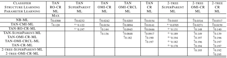
While we have attempted to avoid a proliferation of algorithm names, some name abundance has unavoidably occurred in this paper. We therefore have attempted to use a simple 2-, 3-, or even 4-tag naming scheme where A-B-C-D is such that “A” (if given) refers to either TAN (1-tree) or 2-tree, “B” and “C” refer to the structure learning approach, and “D” (if given) refers to the parameter training method of the final resultant model structure. For the ordering heuristics “B” refers to the ordering method, “C” refers to the parent selection and internal parameter learning strategy. For the remaining structure learning heuristics only “B” is present. Thus, TAN-OMI-CRML-CL would be the OMI procedure for ordering, parent selection evaluated using CR (with ML training used at that time), and with CL used to train the final model which would be a 1-tree (note moreover that TAN-OMI-CR-CL is equivalent since ML is the default training method).
6.1 Experimental Setup
Any continuous features were discretized using recursive minimal entropy partitioning (Fayyad and Irani, 1993) where the codebook is produced using only the training data. This discretization method uses the class entropy of candidate partitions to determine the bin boundaries. The candidate parti-tion with the minimal entropy is selected. This is applied recursively on the established partiparti-tions and the minimum description length approach is used as stopping criteria for the recursive parti-tioning. In Dougherty et al. (1995), an empirical comparison of different discretization methods has been performed and the best results have been achieved with this entropy-based discretization. Throughout our experiments, we use exactly the same data partitioning for each training procedure. We performed simple smoothing, where zero probabilities in the conditional probability tables are
initialized to the values obtained by the ML approach (Greiner et al., 2005). The gradient descent
parameter optimization is terminated usingcross tuning as suggested in Greiner et al. (2005).
6.2 Data Characteristics
In the following, we introduce several data sets used in the experiments.
6.2.1 UCI DATA
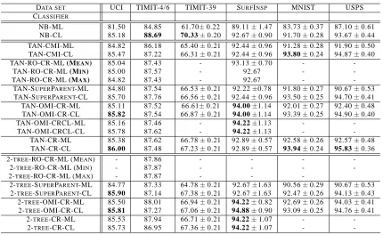
We use 25 data sets from the UCI repository (Merz et al., 1997) and from Kohavi and John (1997). The same data sets, 5-fold cross-validation, and train/test learning schemes as in Friedman et al. (1997) are employed. The characteristics of the data sets are summarized in Table 7 in the Ap-pendix A.
6.2.2 TIMIT-4/6 DATA
This data set is extracted from the TIMIT speech corpus using the dialect speaking region 4 which consists of 320 utterances from 16 male and 16 female speakers. The speech is sampled at 16 kHz. Speech frames are classified into the following classes, voiced (V), unvoiced (U), silence (S), mixed sounds (M), voiced closure (VC), and release (R) of plosives. We therefore are performing frame-by-frame phone classification (contrasted with phone recognition using, say, a hidden Markov model). We perform experiments with only four classes V/U/S/M and all six classes V/U/S/M/VC/R using 110134 and 121629 samples, respectively. The class distribution of the four class experiment V/U/S/M is 23.08%, 60.37%, 13.54%, 3.01% and of the six class case V/U/S/M/VC/R is 20.9%, 54.66%, 12.26%, 2.74%, 6.08%, 3.36%. Additionally, we perform classification experiments on data of male speakers (Ma), female speakers (Fe), and both genders (Ma+Fe). For each gender we have approximately the same number of samples. The data have been split into 2 mutually exclusive subsets of
D
∈ {S
1,S
2}where the size of the training dataS
1is 70% and of the test dataS
2is 30%of
D
. The classification experiments have been performed with 8 wavelet-based features combinedwith 12 mel-frequency cepstral coefficients (MFCC) features, that is, 20 features. More details about the features can be found in Pernkopf et al. (2008). We have 6 different classification tasks
for each classifier, that is, Ma+Fe, Ma, Fe×4 or 6 Classes.
6.2.3 TIMIT-39 DATA
This again is a phone classification test but with a larger number of classes. In accordance with Halberstadt and Glass (1997) we cluster the 61 phonetic labels into 39 classes, ignoring glottal stops. For training, 462 speakers from the standard NIST training set have been used. For testing the remaining 168 speakers from the overall 630 speakers were employed. Each speaker speaks
10 sentences including two sentences which are the same among all speakers (labeled assa), five
sentences which were read from a list of phonetically balanced sentences (labeled as sx), and 3
randomly selected sentences (labeled assi). In the experiments, we only use the sx and si sentences
since thesa sentences introduce a bias for certain phonemes in a particular context. This means that
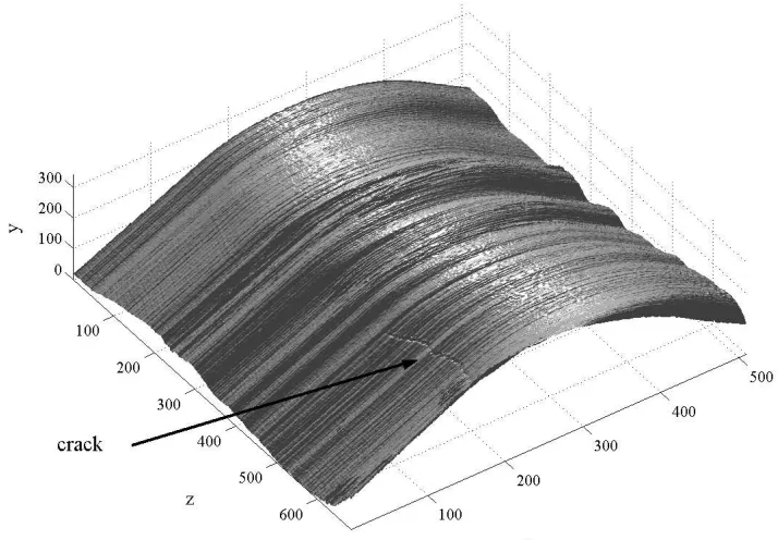
Figure 5: Acquired surface data with an embedded crack.
every 10ms of the utterance with a window size of 25ms. A phonetic segment, which can be variable length, is split at a 3:4:3 ratio into 3 parts. The fixed-length feature vector is composed of: 1) three averages of the 13 MFCC’s calculated from the 3 portions (39 features); 2) the 13 Derivatives of the beginning of the first and the end of the third segment part (26 features); and 3) the log duration of the segment (1 feature). Hence, each phonetic segment is represented by 66 features.
6.2.4 SURFACEINSPECTIONDATA(SURFINSP)
This data set was acquired from a surface inspection task. Surface defects with three-dimensional characteristics on scale-covered steel blocks have to be classified into 3 classes. The 3-dimensional raw data showing the case of an embedded surface crack is given in Figure 5. The data set consists of 450 surface segments uniformly distributed into three classes. Each sample (surface segment) is represented by 40 features. More details on the inspection task and the features used can be found elsewhere (Pernkopf, 2004).
6.2.5 MNIST DATA
We evaluate our classifiers on the MNIST data set of handwritten digits (LeCun et al., 1998) which
contains 60000 samples for training and 10000 digits for testing. The digits are centered in a 28×28
gray-level image. We re-sample these images at a resolution of 14×14 pixels. This gives 196
Figure 6: USPS data.
6.2.6 USPS DATA
This data set contains 11000 handwritten digit images (uniformly distributed) collected from zip
codes of mail envelopes. Each digit is represented as a 16×16 grayscale image, where each pixel
is considered as individual feature. Figure 6 shows a random sample of the data set. We use 8000 digits for training and the remaining images as a test set.
6.3 Conditional Likelihood and Maximum Mutual Information Orderings
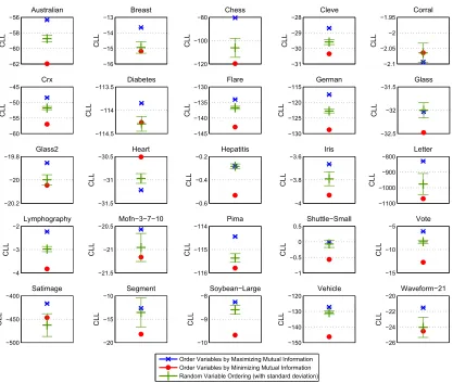
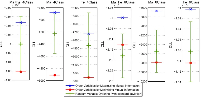
In the following, we evaluate the ordering heuristics using 31 different classification scenarios (from the UCI and the TIMIT-4/6 data sets) comprising differing input features and differing numbers of classes. We compare our ordering procedure (i.e., OMI, where we maximize the mutual informa-tion as in Equainforma-tion 2) with several other possible orderings in an attempt to empirically show that our aforementioned intuition regarding order (see Section 5.1) is sound in the majority of cases. In particular, we compare against an ordering produced by minimizing the mutual information (replac-ing argmax with argmin in Equation 2). Additionally, we also compare against 100 uniformly-at-random orderings. For the selection of the conditioning variables (see Section 5.2) the CL score is used in each case. ML parameter estimation is used for all examples in this section.
Figure 7 and Figure 8 show the resulting conditional log likelihoods (CLL) of the model scoring the training data after the TAN network structures (1-trees in this case) have been determined for the various data sets. As can be seen, our ordering heuristic performs better than both the random and the minimum mutual information orderings on 28 of the 31 cases. The random case shows the
mean and±one standard deviation out of 100 orderings. ForCorral, Glass, and Heart there is no
benefit, but the data sets are on the smaller side where it is less unexpected that generative structure learning would perform better (Ng and Jordan, 2002).