Identification of Recurrent Neural Networks by Bayesian Interrogation Techniques

(1)

Identification of Recurrent Neural Networks by Bayesian

Interrogation Techniques

Department of Information Systems, Eötvös Loránd University Pázmány P. sétány 1/C, Budapest H-1117, Hungary

Editor: Zoubin Ghahramani

Abstract

We introduce novel online Bayesian methods for the identification of a family of noisy recurrent neural networks (RNNs). We present Bayesian active learning techniques for stimulus selection given past experiences. In particular, we consider the unknown parameters as stochastic variables and use A-optimality and D-optimality principles to choose optimal stimuli. We derive myopic cost functions in order to maximize the information gain concerning network parameters at each time step. We also derive the A-optimal and D-optimal estimations of the additive noise that perturbs the dynamical system of the RNN. Here we investigate myopic as well as non-myopic estimations, and study the problem of simultaneous estimation of both the system parameters and the noise. Em-ploying conjugate priors our derivations remain approximation-free and give rise to simple update rules for the online learning of the parameters. The efficiency of our method is demonstrated for a number of selected cases, including the task of controlled independent component analysis.

Keywords: active learning, system identification, online Bayesian learning, A-optimality, D-optimality, infomax control, optimal design

1. Introduction

When studying systems in interactive and online fashion, it is of high relevance to facilitate fast information gain during the interaction (Fedorov, 1972; Cohn, 1994). As an example, consider experiments aiming at the description of the receptive field of different neurons. These experi-ments look for those stimuli that maximize the response of the given neuron (deCharms et al., 1998; Földiák, 2001). Neurons, however, might change due to the investigation, so the minimization of interaction is highly desired. Different techniques have been developed to speed up the identifica-tion procedure. One approach searches for stimulus distribuidentifica-tion that maximizes mutual informaidentifica-tion between stimulus and response (Machens et al., 2005). A recent technique assumes that the un-known system belongs to the family of generalized linear models (Lewi et al., 2007) and treats the parameters as probabilistic variables. Then the goal is to find the optimal stimuli by maximizing mutual information between the parameter set and the system’s response.

This example motivates our interest in active learning (MacKay, 1992; Cohn et al., 1996; Fuku-mizu, 1996; Sugiyama, 2006) of noisy recurrent artificial neural networks (RNNs), when we have the freedom to interrogate the network and to measure its responses.

(2)

In active learning, the training set may be modified by the learning process itself based on the progress experienced so far. The goal of this modification is to maximize the expected improvement of the precision of the estimation. This idea can for example be used to improve generalization capability in regression and classification tasks or to better estimate hidden parameters. Theoretical concepts have been formulated in the fields of Optimal Experimental Design, or Optimal Bayesian Design (Kiefer, 1959; Fedorov, 1972; Steinberg and Hunter, 1984; Toman and Gastwirth, 1993; Pukelsheim, 1993).

Although active learning is in the focus of current research interest, some relevant theoretical issues are still unresolved. While there are promising studies showing that active learning may outperform uniform sampling under certain conditions (Freund et al., 1997; Seung et al., 1992), in other cases it has been proven that active learning has no advantage over non-adaptive algorithms. For example, this is the case in compressed sensing (Castro et al., 2006a) and also for certain function classes in the area of function approximation (Castro et al., 2006b). Even more problematic is the observation that active learning heuristics may be less efficient than uniform sampling in some situations (Schein, 2005).

There are several forms of active learning. The most relevant difference is in the definition of the value of information. One of the simplest heuristics is the Uncertainty Sampling (US): US suggests that in regression or in classification tasks one should choose those training examples, which have the largest uncertainty in the value of the function or in the label of the class, respectively (Lewis and Catlett, 1994; Lewis and Gale, 1994; Cohn et al., 1996). Although several US versions exist with different measure of the uncertainty itself, they all lack robustness. The Query by Committee method improves upon robustness (Seung et al., 1992; Freund et al., 1997): the committee of a few models are trained on the existing training set and the next query points are selected to reduce the disagreement among these models. The method of Roy and McCallum (2001) minimizes the direct error, that is, it tries to choose training points to minimize the expected classification error directly.

In the literature there are other approaches, including decision theory based methods. The orig-inal ideas were worked out in Raiffa and Schlaifer (1961) and Lindley (1971). The objective in this method family is to choose the design such that the predicted value of a given utility function become maximal. Numerous utility functions have been proposed. For example, if we aim to

esti-mate the unknown parameterθ, then one possible direction is the minimization of, for example, the

entropy or the standard deviation of the posterior distribution. If we minimize the entropy then we arrive at the D-optimality principle (Bernardo, 1979; Stone, 1959). This principle is equivalent to the information maximization method (also known as infomax principle) of Lewi et al. (2007). If we intend to minimize the standard deviation then the result is the A-optimality principle (Duncan and DeGroot, 1976). A special case is called the c-optimality principle (Chaloner, 1984) when the

goal is to estimate a linear projection of parameterθ(cTθ). There exist a number of other methods,

called alphabetical optimality and utility functions. For a review see, for example, Chaloner and Verdinelli (1995). Although the original ideas belong to the field of optimal experimental design, they have appeared also in active learning recently (MacKay, 1992; Tong and Koller, 2000; Schein and Ungar, 2007).

(3)

learning the parameters and structure of Bayes nets (Tong and Koller, 2000, 2001a) and Hidden Markov Models (Anderson and Moore, 2005).

Our framework is similar to the generalized linear model (GLM) approach used by Lewi et al. (2007): we would like to choose interrogating, or ‘control’ inputs in order to (i) identify the pa-rameters of the network and (ii) estimate the additive noise efficiently. From now on, we use the terms control and interrogation interchangeably; control is the conventional expression, whereas the word interrogation expresses our aims better. We apply online Bayesian learning (Opper and Winther, 1999; Solla and Winther, 1999; Honkela and Valpola, 2003; Ghahramani, 2000). For Bayesian methods, prior updates often lead to intractable posterior distributions such as a mixture of exponentially numerous distributions. Here, we show that, for the model studied in this paper, computations are both tractable and approximation-free. Further, the emerging learning rules are simple. We also show that different stimuli are needed for the same RNN model depending on whether the goal is to estimate the weights of the RNN or the additive perturbation (referred to as ‘driving noise’).

In this article we investigate the D-optimality, as well as the A-optimality principles. To the best of our knowledge, neither of them has been applied to the typical non-spiking stochastic artificial recurrent neural network model that we treat here.

The contribution of this paper can be summarized as follows: We use A-optimality and D-optimality principles and derive cost functions and algorithms for (i) the learning of parameters of the stochastic RNN and (ii) the estimation of its driving noise. We show that, (iii) using the D-optimality interrogation technique, these two tasks are incoherent in the myopic (i.e., single step look-ahead) control scheme: signals derived from this principle for parameter estimation are sub-optimal (basically the worst possible) for the estimation of the driving noise and vice versa. (iv) We show that for the case of noise estimation task the two principles, that is, A- and D-optimality principles result in the same cost function. (v) For the A-optimality case, we derive equations for the joined estimation of the noise and the parameters. On the contrary, we show also that (vi) D-optimality cannot be applied on the same joined task. For the case of noise estimation, (vii) a non-myopic multiple step look-ahead heuristics is introduced and we demonstrate its applicability through numerical experiments.

(4)

2. The Model

Let P(e) =

N

e(m,V)denote the probability density of a normally distributed stochastic variable e

with mean m and covariance matrix V. Let us assume that we have d simple computational units called ‘neurons’ in a recurrent neural network:

rt+1 = g

I

∑

i=0

Firt₋i+ J

∑

j=0

Bjut+1₋j+et+1

!

, (1)

where _{et}, the driving noise of the RNN, denotes temporally independent and identically

dis-tributed (i.i.d.) stochastic variables and P(et) =

N

et(0,V), rt∈R

d_{represents the observed activities}

of the neurons at time t. Let ut ∈Rc denote the control signal at time t. The neural network is

formed by the weighted delays represented by matrices Fi(i=0, . . . ,I) and Bj( j=0, . . . ,J), which connect neurons to each other and also the control components to the neurons, respectively. Control can also be seen as the means of interrogation, or the stimulus to the network (Lewi et al., 2007).

We assume that function g :Rd→Rd in (1) is known and invertible. The computational units, the

neurons, sum up weighted previous neural activities as well as weighted control inputs. These sums are then passed through identical non-linearities according to Eq. (1). Our goal is to estimate the parameters Fi∈Rd×d (i=0, . . . ,I), Bj∈Rd×c( j=0, . . . ,J) and the covariance matrix V, as well

as the driving noise et by means of the control signals.

In artificial neural network terms, (1) is in the form of rate code models. This is the typical form for RNNs, but there are methods to approximate rate code description with spike codes and vice versa. For the case of RNNs, the best is to compare Liquid State Machine, a spike code model of Maass et al. (2002) with the Echo State Network, the corresponding rate code model of Jaeger (2001). Rate code, very crudely, is the low pass filtered spike code, whereas spike code can be seen as the response of integrate-and-fire neurons. We show that analytic cost functions emerge for the rate code RNN model. Due to the applied conjugate priors, we can calculate the high dimensional integrals involved in our derivations, and hence these derivations remain approximation-free and give rise to simple update rules.

3. Bayesian Approach

Here we embed the estimation task into the Bayesian framework. First, we introduce the follow-ing notations: xt+1= [rt−I;. . .; rt; ut−J+1;. . .; ut+1], yt+1=g−1(rt+1), A= [FI, . . . ,F0,BJ, . . . ,B0]∈

Rd×m. With these notations, model (1) reduces to a linear equation

yt = Axt+et. (2)

In order to estimate the unknown quantities (parameter matrix A, noise et and its covariance matrix

V) in an online fashion, we rely on Bayes’ method. We assume that prior knowledge is available

(5)

1999). In order to avoid approximations, we apply the method of conjugated priors (Gelman et al., 2003). For matrix A we assume a matrix valued normal distribution prior.

For the case of D-optimality principle, we shall use the inverted Wishart (IW) distribution as our prior for covariance matrix V. This is the most general known conjugate prior distribution for the covariance matrix of a normal distribution at present. For A-optimality, however, we keep the derivations simple and assume that the covariance matrix has diagonal structure. In turn, we replaced the IW assumption on the prior with the distribution of the Product of Inverted Gammas (PIG).

We define the normally distributed matrix valued stochastic variable A_∈Rd×m by using the

following quantities: M_∈Rd×m _{is the expected value of A. V}_∈_Rd×d _{is the covariance matrix}

of the rows, and K_∈Rm×m is the so-called precision parameter matrix that we shall modify in

accordance with the Bayesian update. Matrix K contains the estimations of the ‘Bayesian trainer’ about the precision of parameters in A. Informally, matrix K behaves as the inverse of a covariance matrix. Upon each observation, matrix K is updated. The larger the eigenvalues of this matrix, the smaller the variance ellipsoids of the posteriori estimations are.

Both K and V are positive semi-definite matrices. The density function of the stochastic variable

A is defined as:

N

A(M,V,K) = |

K_|d/2

|2πV_|m/2exp(−

1

2tr((A−M)

T_V₋1₍_A

−M)K)),

where tr, _{| · |}, and superscript T denote the trace operation, the determinant, and transposition,

respectively (see, e.g., Gupta and Nagar, 1999; Minka, 2000). We assume that Q_∈Rd×dis a positive

definite matrix and n>0. Using these notations, the density of the Inverted Wishart distribution with parameters Q and n is as follows (Gupta and Nagar, 1999):

I W

V(Q,n) =

1

Zn,d 1

|V_|(d+1)/2

V−1Q

2

n/2

exp(₋1

2tr(V

−1_Q₎₎_,

where Zn,d=πd(d−1)/4 d

∏

i=1

Γ((n+1−i)/2)andΓ(.)denotes the gamma function.

Similarly, let V=diag(v)_∈Rd×ddiagonal covariance matrix with 0<v_∈Rddiagonal values.

With the slight abuse of notation we will use later the v=diag(V)_∈Rdterm, too. Then the density

of PIG is defined as

P I G

_V(α,β) =

d

∏

i=1

βαi

i

Γ(αi)

v−αi−1

i exp(−

βi

vi

),

whereαi>0 andβi>0 are the shape and scale parameters respectively. Now, one can rewrite model (2) as follows:

P(A_|V) =

N

A(M,V,K), (3) P(et|V) =

N

et(0,V), (4) P(yt|A,xt,V) =

N

yt(Axt,V), (5)

and P(V) =

P I G

_V(α,β) or P(V) =

I W

V(Q,n) depending on whether we want to use A- or

(6)

4. D-Optimality Approach for Parameter Learning

Let us compute the D-optimal parameter estimation strategy for our RNN given by (1) and rewritten into (3)-(5). Let us introduce two shorthands; θ=_{A,V_}, and _{x_}_ij =_{xi, . . . ,xj}. We choose the control value in (1) at each instant to provide maximal expected information concerning the

unknown parameters. Assuming that_{x_}t₁,_{y_}t₁are given, according to the infomax principle our

goal is to compute

arg max

ut+1

I(θ,yt+1;{x}1t+1,{y}t1), (6)

where I(a,b; c)denotes the mutual information of stochastic variables a and b for fixed parameters

c. Let H(a_|b; c)denote the conditional entropy of variable a conditioned on variable b and for fixed parameter c. Note that

I(θ,yt+1;{x}t1+1,{y}

t

1) =H(θ;{x}t1+1,{y}

t

1)−H(θ|yt+1;{x}t1+1,{y}

t

1),

holds (Cover and Thomas, 1991) and H(θ;_{x_}₁t+1,_{y_}t₁) =H(θ;_{x_}₁t,_{y_}t₁) is independent from

ut+1, hence our task is reduced to the evaluation of the following quantity:

arg min

ut+1

H(θ_|yt+1;{x}1t+1,{y}t1) = (7)

=arg min

ut+1−

Z

dyt+1P(yt+1|{x}t₁+1,{y}t1)

Z

dθP(θ_|{x_}₁t+1,_{y_}t₁+1)log P(θ_|{x_}t₁+1,_{y_}t₁+1).

In order to solve this minimization problem we need to evaluate P(yt+1|{x}t1+1,{y}t1), the posterior P(θ_|{x_}t₁+1,_{y_}t₁+1), and the entropy of the posterior, that is R

dθP(θ_|{x_}₁t+1,_{y_}t₁+1)

log P(θ_|{x_}t₁+1,_{y_}t₁+1), where P(a_|b)denotes the conditional probability of variable a given con-dition b. The main steps of these computations are presented below.

Assume that the a priori distributions P(A_|V,_{x_}t₁,_{y_}t₁) =

N

(A_|Mt,V,Kt) and

P(V_|{x_}t₁,_{y_}₁t) =

I W

V(Qt,nt)are known. Then the posterior distribution ofθis:

P(A,V_|{x_}₁t+1,_{y_}t₁+1) = P(yt+1|A,V,xt+1)P(A|V,{x}

t

1,{y}t1)P(V|{x}t1,{y}t1) P(yt+1|{x}₁t+1,{y}t₁)

,

=

N

yt+1(Axt+1,V)

N

A(Mt,V,Kt)

I W

V(Qt,nt)

R

A

R

V

N

yt+1(Axt+1,V)

N

A(Mt,V,Kt)

I W

V(Qt,nt) .

This expression can be rewritten in a more useful form: let K_∈Rm×m and Q_∈Rd×d be positive

definite matrices. Let A_∈Rd×m, and let us introduce the density function of the matrix valued

Student-t distribution (Kotz and Nadarajah, 2004; Minka, 2000) as follows:

T

A(Q,n,M,K) =|

K_|d/2

πdm/2 Zn+m,d

Zn,d

|Q_|n/2

|Q+ (A−M)K(A−M)T_|(m+n)/2.

Now, we need the following lemma:

Lemma 4.1

N

y(Ax,V)

N

A(M,V,K)

I W

V(Q,n) =

N

A((MK+yxT)(xxT+K)−1,V,xxT+K)×

×

I W

V

Q+ (y₋Mx) (1₋xT(xxT+K)−1x) (y₋Mx)T,n+1

× ×

T

y Q,n,Mx,1−xT(xxT+K)−1x

(7)

The proof can be found in the Appendix.

Using this lemma, we can compute the posterior probabilities. We introduce the following quantities:

γt+1 = 1−xTt+1(xt+1xTt+1+Kt)−1xt+1, (8) nt+1 = nt+1,

Mt+1 = (MtKt+yt+1xTt+1)(xt+1xTt+1+Kt)−1, (9) Qt+1 = Qt+ (yt+1−Mtxt+1)γt+1(yt+1−Mtxt+1)T. (10)

For the posterior probabilities we have determined that

P(A_|V,_{x_}₁t+1,_{y_}t₁+1) =

N

A(Mt+1,V,xt+1xTt+1+Kt), (11)

P(V_|{x_}t₁+1,_{y_}₁t+1) =

I W

V(Qt+1,nt+1), (12) P(yt+1|{x}t1+1,{y}

t

1) =

T

yt+1(Qt,nt,Mtxt+1,γt+1).

Now we are in the position to compute the entropy of the posterior distribution ofθ=_{A,V_}using

the following lemma:

Lemma 4.2 The entropy of a stochastic variable with density function P(A,V) =

N

A(M,V,K)

I W

V(Q,n)assumes the form−d₂ln|K|+ (m+₂d+1)ln|Q|+f1,1(d,n), where f1,1(d,n) depends only on d and n.

Lemmas 4.1 and 4.2 lead to the following corollary:

Corollary 4.3 For the entropy of a stochastic variable with posterior distribution P(A,V_|x,y) it holds that

H(A,V; x,y) =₋d

2ln|xx

T₊_K

|+f1,1(d,n) + (

m+d+1

2 )ln|Q+ (y−Mx)γ(y−Mx)

T |.

We note that the following lemma also holds:

Lemma 4.4

Z

T

y(Q,n,µ,γ)ln|Q+ (y−µ)γ(y−µ)T|dy

is independent from bothµandγ,

and thus we can compute the conditional entropy expressed in (7):

Lemma 4.5

H(A,V|y; x) =

Z

p(y|x)H(A,V; x,y)dy=₋d

2ln|xx

T₊_K_|₊_f1

,2(Q,n,m),

(8)

Collecting all the terms, we arrive at the following intriguingly simple expression

u_topt₊₁ = arg min

ut+1

Z

p yt+1|{x}t₁+1,{y}t1

H(A,V_|{x_}t₁+1,_{y_}t₁,yt+1)dyt+1,

= arg min

ut+1− d

2ln|xt+1x T

t+1+Kt|=arg max

ut+1

xT_t₊₁K−_t 1xt+1, (13)

where

xt+1= [. rt−I;. . .; rt; ut−J+1;. . .; ut+1],

and we used that _|xxT+K_|=_|K_|(1+xTK−1x) according to the Matrix Determinant Lemma

(Harville, 1997). We assume a bounded domain

U

for the control, which is necessary to keep

the maximization procedure of (13) finite. This is, however, a reasonable condition for all practical applications. So,

u_topt₊₁=arg max

ut+1∈U

xT_t₊₁K−_t 1xt+1, (14)

In what follows D-optimal control will be referred to as ‘infomax interrogation scheme’. The steps of our algorithm are summarized in Table 1.

Control Calculation

ut+1=arg maxu∈UˆxtT+1Kt−1ˆxt+1

where ˆxt+1= [rt−I;. . .; rt; ut−J+1;. . .; ut; u] set xt+1= [rt−I;. . .; rt; ut−J+1;. . .; ut; ut+1]

Observation

observe rt+1, and let yt+1=g−1(rt+1)

Bayesian update

Mt+1= (MtKt+yt+1xTt+1)(xt+1xtT+1+Kt)−1 Kt+1=xt+1xTt+1+Kt

nt+1=nt+1

γt+1=1−xtT+1(xt+1xTt+1+Kt)−1xt+1

Qt+1=Qt+ (yt+1−Mtxt+1)γt+1(yt+1−Mtxt+1)T

Table 1: Pseudocode of the algorithm

Computation of the inverse(xt+1xTt+1+Kt)−1in Table 1 can be simplified considerably by the

following recursion: let Pt =K−t 1, then according to the Sherman-Morrison formula (Golub and

Van Loan, 1996)

Pt+1= (xt+1xTt+1+Kt)−1=Pt−

Ptxt+1xTt+1Pt 1+xT

t+1Ptxt+1

. (15)

In this expression matrix inversion disappears and only a real number is inverted instead.

5. A-Optimality Approach for Parameter Learning

(9)

u_topt₊₁=arg min

ut+1

Z

dyt+1P(yt+1|{x}t1+1,{y}t1)trVar[θ|{x}t1+1,{y}t1+1]. (16)

where Var[θ_|

F

]denotes the conditional covariance matrix ofθgiven the condition

F

.

To keep the calculations simple, in this case we use

P I G

_V(αt,βt)prior distribution for the co-variance matrix instead of

I W

V(Qt,nt). Using the notations of (8)-(10), the posterior distributions assume the following forms:

Lemma 5.1

P(A_|V,_{x_}t₁+1,_{y_}t₁+1) =

N

A(Mt+1,V,xt+1xtT+1+Kt), (17)

P(V_|{x_}t₁+1,_{y_}₁t+1) =

P I G

_V(αt+1,βt+1), P(yt+1|{x}t1+1,{y}

t

1) =

d

∏

i=1

T

(yt+1)i

(βt)i,2(αt)i,(Mtxt+1)i,

γt+1

2

, (18)

where we used the shorthands

(αt+1)i = (αt)i+1/2,

(βt+1)i = (βt)i+ ((yt+1)i−(Mtxt+1)i)2

γt+1

2 . (19)

Given that P(V_|{x_}t₁+1,_{y_}t₁+1) belongs to the

P I G

family we can calculate the quantity

Var(V_|{x_}t₁+1,_{y_}t₁+1)(Gelman et al., 2003):

tr Var[V_|{x_}t₁+1,_{y_}t₁+1] =

d

∑

i=1

(βt+1)i

((αt+1)i−1)2((αt+1)i−2)

.

We will need the following lemma:

Lemma 5.2

tr Var[A_|{x_}t₁+1,_{y_}t₁+1]

= tr Kt+xt+1xtT+1

−1

E[trV_|{x_}t₁+1,_{y_}t₁+1],

= tr Kt+xt+1xtT+1

−1 d

∑

i=1

(βt+1)i

(αt+1)i−1

.

Now we can elaborate on the A-optimal cost function for parameter estimation (16):

Z

dyt+1P(yt+1|{x}t1+1,{y}1t)trVar[θ|{x}1t+1,{y}t1+1] = (20)

=

Z

dyt+1

d

∏

i=1

T

(yt+1)i

(βt)i,2(αt)i,(Mtxt+1)i,

γt+1

2

×

× tr Kt+xt+1xTt+1

−1 d

∑

i=1

(βt+1)i

(αt+1)i−1

+

d

∑

i=1

(βt+1)i

((αt+1)i−1)2((αt+1)i−2) !

,

= tr

Kt+xt+1xTt+1

−1

(10)

where f2,1and f2,2depend only onαt+1, andβt. Here we used (18), (19) and Lemma 4.4.

Applying again the Sherman-Morrison formula (15) and the fact that tr[K−t 1xt+1x_tT₊₁K−t 1] =

tr[x_tT₊₁K−t 1K−t 1xt+1],we arrive at the following expression for A-optimal parameter estimation:

u_topt₊₁=arg max

ut+1∈U

xT_t₊₁K_t−1K−_t 1xt+1

1+xT

t+1Kt−1xt+1

, (21)

which is a hyperbolic programming task.

We can conclude that while in the D-optimality case the task is to minimize expression_|(Kt+

xt+1xTt+1)−1|, the A-optimality principle is concerned with the minimization of tr[(Kt+xt+1xTt+1)−1].

6. D-Optimality Approach for Noise Estimation

One might wish to compute the optimal control for estimating noise et in (1), instead of the

identi-fication problem above. Based on (1) and because

et+1=yt+1−

I

∑

i=0

Firt₋i− J

∑

j=0

Bjut+1₋j, (22)

one might think that the best strategy is to use the optimal infomax control of Table 1, since it provides good estimations for parameters A= [FI, . . . ,F0,BJ, . . . ,B0]and so for noise et.

Another—and different—thought is the following. At time t+1, let the estimation of the noise

be ˆet+1 =yt+1−∑iI=0Fˆtirt−i−∑Jj=0Bˆtjut+1−j, where ˆFti (i=0,. . . ,I), and ˆBtj (j=0,. . . ,J) denote the estimations of F and B respectively.

Using (22), we have that

et+1−ˆet+1=

I

∑

i=0

(Fi−Fˆti)rt−i+ J

∑

j=0

(Bj−Bˆtj)ut+1−j. (23)

This hints that the control should be ut=0 for all times in order to get rid of the error contribution

of matrix Bj in (23).

Straightforward D-optimality considerations oppose the utilization of objective (6) for the present task. One can optimize, instead, the following quantity:

arg max

ut+1

I(et+1,yt+1;{x}t₁+1,{y}t1).

In other words, for the estimation of the noise we want to design a control signal ut+1such that the

next output is the best from the point of view of greedy optimization of mutual information between the next output yt+1and the noise et+1. It is easy to show that this task is equivalent to the following

optimization problem:

arg min

ut+1

Z

dyt+1P(yt+1|{x}t1+1,{y}t1)H(et+1;{x}1t+1,{y}t1+1), (24)

where H(et+1;{x}t1+1,{y}

t+1

1 ) =H(Axt+1;{x}t1+1,{y}

t+1

1 ), because et+1=yt+1−Axt+1.

In practice, we perform this optimization in an appropriate domain

U

. After some mathematical

(11)

Lemma 6.1

u_topt₊₁=arg min

ut+1∈U

xT_t₊₁K−_t 1xt+1. (25)

The proof of this lemma can be found in the Appendix.

It is worth noting that this D-optimal cost function for noise estimation and the D-optimal cost function derived for parameter estimation in (13) are not compatible with each other. Estimating one of them quickly will necessarily delay the estimation of the other.

We shall show later (Section 9) that for large t values, expression (25) gives rise to control values close to ut =0.

7. A-Optimality Approach for Noise Estimation

Instead of (24), our task is to compute the following quantity:

arg min

ut+1

Z

dyt+1P(yt+1|{x}t1+1,{y}t1)tr Var[et+1|{x}1t+1,{y}t1+1]

. (26)

We will apply the identity

N

Axt+1

Mt+1xt+1,V, xtT+1Kt−+11xt+1

−1

P I G

_V(αt+1,βt+1) =

=

d

∏

i=1

T(

Axt+1)i



(βt+1)i,2(αt+1)i,(Mt+1xt+1)i, xtT+1

K−_t₊1₁

2 xt+1

!−1

×

×

P I G

_Vαt+1+1,βt+1+diag[(yt+1−Mtxt+1)

γt+1

2 (yt+1−Mtxt+1) T_]_,

which can be proven by using Lemma A.1. We can simplify (26) by noting that

tr Var[et+1|{x}t1+1,{y}

t+1 1 ]

=tr Var[Axt+1|{x}t1+1,{y}

t+1 1 ]

.

We also take advantage of the fact that

VarV[E[Axt+1|V,{x}t1+1,{y}t1+1]] =VarV[Mt+1xt+1] =0,

and proceed as

EV[trVar(Axt+1|V,{x}t₁+1,{y}₁t+1)] = EV[tr(V⊗xTt+1Kt−+11xt+1|{x}

t+1 1 ,{y}

t+1 1 ],

= tr(E[V_|{x_}t₁+1,_{y_}₁t+1])xT_t₊₁K−_t₊1₁xt+1,

= xT_t₊₁K−_t₊1₁xt+1

d

∑

i=1

(βt+1)i

(αt+1)i−1

,

where_⊗denotes the Kronecker product. The law of total variance says that

Var[Ax] =Var[E[Ax_|V]] +E[Var[Ax_|V]],

and hence

trVar[Axt+1|{x}t₁+1,{y}₁t+1] =xTt+1Kt−+11xt+1

d

∑

i=1

(βt+1)i

(αt+1)i−1

(12)

There is another way to arrive at the same result. One can apply (37) with Lemma A.1 and use the fact that the covariance matrix of a

T

x(β,α,µ,K)distributed variable is βK

−1

α−2 (Gelman et al.,

2003). That is, we have

trVar[Axt+1|{x}1t+1,{y}t1+1] =

d

∑

i=1



  

(βt+1)i

xT t+1

K−_t₊1₁ 2 xt+1

2(αt+1)i−2



  

.

Now, we can proceed as

Z

dyt+1P(yt+1|{x}t1+1,{y}

t

1)tr Var[et+1|{x}t1+1,{y}

t+1 1 ]

= (27)

Z

dyt+1P(yt+1|{x}t₁+1,{y}t1)tr(E[V|{x}t1+1,{y}

t+1 1 ])x

T

t+1K−t+11xt+1 =

xT_t₊₁K_t−₊1₁xt+1

Z

dyt+1P(yt+1|{x}t1+1,{y}t1)

d

∑

i=1

(βt+1)i

(αt+1)i−1

=

xT_t₊₁K−_t₊1₁xt+1

d

∑

i=1

f4((αt+1)i,(βt)i),

where we used (18), (19) and Lemma 4.4 again. Applying the Sherman-Morrison formula one can see that the task is the same as in (25).

8. Joint Parameter and Noise Estimation

So far we wanted to optimize the control in order to speed-up learning of either the parameters of the dynamics or the noise. In this section we investigate the A- and D-optimality principles for the joint parameter and noise estimation task.

8.1 A-optimality

According to the A-optimality principle, the joined objective for parameter and noise estimation is given as:

Z

dyt+1P(yt+1|{x}1t+1,{y}t1)trVar[vec(A),diag(V),et+1|{x}1t+1,{y}t1+1].

By means of (20), (27) and Lemma 5.2, it is equivalent to:

Z

dyt+1P(yt+1|{x}t1+1,{y}t1)E[trV|x1t+1,yt1+1]tr

Kt+xt+1xTt+1

−1

+xT_t₊₁K_t−₊1₁xt+1

.

From here, one can prove the following lemma in a few steps:

Lemma 8.1 The A-optimality principle in the joined parameter and noise estimation task gives rise

to the following choice for control:

uopt_t₊₁=arg max

ut+1∈U

1+x_tT₊₁Kt−1K−t 1xt+1

1+xT_t₊₁Kt−1xt+1

. (28)

(13)

8.2 D-optimality

One of the most salient differences between A-optimality and D-optimality is that for D-optimality we have

H(X,Y) =H(X_|Y) +H(Y),

however, for A-optimality the corresponding equation does not hold in general, because:

trVar(X,Y)₆=EY[trVar(X|Y)] +trVar(Y).

An implication—as we shall see below—is that we cannot use the D-optimality principle for the joint parameter and noise estimation task. For D-optimality our cost function would be

arg min

ut+1

Z

dyt+1P(yt+1|{x}₁t+1,{y}t1)H(A,V,et+1|{x}t₁+1,{y}t₁+1),

but the following equality holds:

H(A,V,et+1|{x}t1+1,{y}t1+1) =H(A,V|{x}1t+1,{y}1t+1) +H(et+1|A,V{x}t1+1,{y}t1+1),

and since et+1=yt+1−Axt+1, therefore the last term H(et+1|A,V{x}t₁+1,{y}t₁+1) =−∞. The first

term is a finite real number, thus we can conclude that the D-optimality cost function is constant

−∞, and therefore the D-optimality principle does not suit the joint parameter and noise estimation

task.

9. Non-myopic Optimization

Until now, we considered myopic methods for the optimization of control, that is, we aimed to determine the optimum of the objective only for the next step. In this section, we show a non-myopic heuristics for the noise estimation task (25).

The optimization of the derived objective function, xT_t₊₁Kt−1xt+1, is simple, provided that Kt is fixed during the optimization of ut+1. If so, then the optimization task is quadratic. To see this, let

us partition matrix Kt as follows:

Kt=

K11_t K_t12 K21_t K_t22

,

where K11

t ∈Rd×d,K21t ∈Rm−d×d, Kt22∈Rm−d×m−d. It is easy to see that if domain

U

in (25) is large enough then

u_topt₊₁= (K_t22)−1K21_t rt. (29) It occurs, however, that the objective xT_t₊₁Kt−1xt+1 may be improved by considering

multiple-step lookaheads. In this case matrix Ktcan be subject to changes in xT_t₊₁Kt−1xt+1, because it depends

on previous control inputs u1, . . . ,ut derived from previous optimization steps.

We propose a two-step heuristics for the long-term minimization of expression xT_t₊₁K−t 1xt+1.

During the firstτ-step long stage, we focus only on the minimization of the quantity_|K−_t 1_|. Then,

if this quantity _|Kt−1| becomes small, we start the second stage: we consider K−t 1 as given and

(14)

this method ‘sacrifices’ the firstτsteps in order to achieve smaller costs later; this heuristic

opti-mization is non-myopic. More formally, we use the strategy of Table 1 in the firstτsteps in order to

decrease quantity_|K−_t 1_|fast. Then after thisτ-steps, we switch to the control method of (29). This will decrease the cost function (25) further. We will call this non-greedy interrogation heuristics

introduced for noise estimation ‘τ-infomax noise interrogation’. This non-myopic heuristics admits

that parameter estimation of the dynamics is the prerequisite of noise estimation, because improper

parameter estimation makes apparent noise, and thus the heuristics sacrificesτsteps for parameter

estimation.

In Section 10 we will empirically show that using this non-myopic strategy, afterτsteps we can

achieve smaller cost values in (25)—as well as better performance in parameter estimation—than

using the greedy competitors. The compromise is that in the first τsteps the performance of the

non-myopic control can be worse than that of the other control methods.

We note that in the τ-infomax noise interrogation, for large switching timeτ and for large t

values, _|K22

t |will be large, and hence—according to (29)—the optimal ut for interrogation will

be close to 0. (In Section 10 we will show this empirically.) A reasonable approximation of the

‘τ-infomax noise interrogation’ is to use the control given in Table 1 forτsteps and to switch to

zero-interrogation onwards. This scheme will be called the ‘τ-zero interrogation’ scheme.

10. Numerical Illustrations

We illustrate by numerical simulations the power of A- and D-optimizations.

10.1 Generated Data

This section provides numerical experiments for parameter and noise estimations on artificially generated toy problems.

10.1.1 PARAMETERESTIMATION

We investigated the parameter estimation capability of the D- and A-optimal interrogation. Matrix

F_∈Rd×dhas been generated as a random orthogonal matrix multiplied by 0.9 so that the magnitudes

of its eigenvalues remained below 1. Random matrix B_∈Rd×cwas generated from standard normal

distribution. Elements of the diagonal covariance matrix V of noise et were generated from the

uniform distribution over[0,1]. The process is stable under these conditions.

To study whether or not the D- and A-optimal interrogations are able to estimate the true pa-rameters we measured the averages of the squared deviations of the true matrices F and B and the means of their posterior estimations, respectively. The square roots of these estimations are the

mean squared errors (MSE). One might use other options to measure performance. For example, L2

norm could be replaced by the L1norm and the variance of the posterior estimations could also be

added as the complementary information for the bias.

We examined the following strategies: (i) D-optimal control of Table 1 with

U

= [₋δ,δ]c_{, which}

defines a c-dimensional hypercube. The value ofδwas set to 50. (ii) A-optimal control of (21) with

(15)

For solving the quadratic problem of (14) and (25) we used a subspace trust-region procedure, which is based on the interior-reflective Newton method described by Coleman and Li (1996). Its implementation is available in the Matlab Optimization toolbox. However, the optimization task in (21) is more involved: Generally, the optimization of a constrained hyperbolic programming task is quite difficult. We tried the gradient ascent method, but its convergence appeared to be very slow and we got poor results. In this case, it was more efficient to apply a simplex method as follows:

we know that the optimal solution of (21) lies at the boundary of

U

. Thus, we chose one corner

of hypercube

U

randomly with uniform distribution and moved greedily to the neighboring corners

with the best improvement in the objective. This procedure was iterated until convergence. The method was efficient for our special simple optimization domain.

We investigated two distinct cases. In the first case we set d =10<c=40; the dimension of

the observations is smaller than the dimension of the control. By contrast, in the other case we set

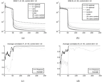
d=40>c=10. Results are shown in Fig. 1 (a-b) and in Fig. 2 (a-b). We separated the MSE values

of matrices B and F. According to the figure, zero control may give rise to early and sudden drops in the MSE values of matrix F. Not surprisingly, however, zero control is unable to estimate matrix

B. For both types of matrices as well as for d<c and for d>c, the D-optimal procedure produced

the smallest MSE after about 50 online estimations, but the A-optimal method reached very similar

levels only a few iterations later. As can be expected,τ-zero control, which is identical to D-optimal

control in the firstτ steps fell behind D-optimal control afterτ since it changes the objective and

estimates the noise and not the parameters afterwards.

For statistical significance studies, we introduced the concept of average correlation curves. We use Fig. 1 to explain this concept. There are 7 curves in Fig. 1 each representing the averages of 25 computer runs. Error bars make the curves incomprehensible and they hide the correlations that may be present between the errors. We note that the relative order of the curves is of interest for us. However, it is possible that in each run the relative order of the curves was the same and the overlap of the error bars—which originates from the large differences between the individual runs—hides this important piece of information. We treat this problem as follows. In each time

instant 1_≤t_≤250 and for all 1_≤i< j_≤25 we compute the empirical (linear, or rank) correlation

of the 7 curves of the ith and jth experiment and take the average of the 25_×24/2=300 values.

The most significant case gives rise to 1 for each of the 300 correlations, that is, the 25 experiments agree in the height of the curves at that time instant, or in their relative orderings for the case of rank correlation. If there is any single experiment out of 25 that produces different heights or orders then the average correlation becomes smaller than 1. For randomly chosen curves the average correlation is 0. Results can be seen in Fig. 1 (c-d) and Fig. 2 (c-d) for linear Pearson and for Kendal rank correlations, respectively. The curves demonstrate that after about 50 steps, the correlations, in particular the linear correlation is almost 1. This means that the curves behaved similarly in a considerable portion of the experiments. The slightly different picture shown by the linear correlation and the rank correlation could be due to the fact that the performance of the A and D-optimal control is very similar after some time, and their ordering may change often, thus giving rise to changes in the ranks in different experiments.

10.1.2 NOISEESTIMATIONS

(16)

0 50 100 150 200 250 10−2

100 102 104

MSE F, d= 40, control dim= 10 D−optimal A−optimal zero random noise 25−zero control 75−zero control

(a)

0 50 100 150 200 250 10−2

100 102 104

MSE B, d= 40, control dim= 10

D−optimal A−optimal zero random noise 25−zero control 75−zero control

(b)

0 50 100 150 200 250 0.2

0.4 0.6 0.8 1

Average correlation F, d= 40, control dim= 10

Pearson Kendall

(c)

0 50 100 150 200 250 0.5

0.6 0.7 0.8 0.9 1

Average correlation B, d= 40, control dim= 10

Pearson Kendall

(d)

Figure 1: Mean Square Error of the estimated parameters for different control strategies and the sig-nificance of the curves. Magnitude of MSE as a function of time is averaged for 25 runs. Dimension of the control is 10. F_∈R40×40, B_∈R40×10. (a): MSE of the estimated matrix ˆF. (b): MSE of the

estimated matrix ˆB. (c): The average correlation curves for the estimation of F. (d): The average

correlation curves for the estimation of B. For details see the text.

We investigated the noise estimation capability of the interrogation in (25) for four cases. The

first set of experiments illustrates that the estimation of driving noise et for large τvalues barely

differs if we replace theτ-infomax noise interrogation with theτ-zero interrogation scheme.

Pa-rameters were the same as above and the MSE of the noise estimation was computed. Results are

shown in Fig. 3: for the case ofτ=21, cost function (25) of theτ-zero interrogation is higher than

that ofτ-infomax interrogation. However, for valuesτ=51 and 81 the performances of the two

schemes are approximately identical. Given thatτ-zero andτ-infomax noise interrogation behave

similarly for largeτvalues, we compare theτ-zero interrogation scheme with other schemes in our

numerical experiments.

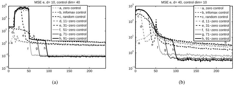
In the second experiment we investigated the problem of noise estimation on a toy problem. Parameters were set as in Section 10.1.1, and the following strategies were compared: zero control,

infomax control, random control and τ-zero control for different τ values. Results are shown in

Fig. 4. It is clear from the figure that neither the zero control, nor the infomax (D-optimal) control

of Table 1 work for this case. If we want to have minimal MSE in approximatelyτsteps then the

best strategy is to apply theτ-zero strategy, that is, the strategy of Table 1 up to τsteps and then

(17)

0 50 100 150 200 250 10−4

10−2 100 102 104

MSE F, d= 10, control dim= 40 D−optimal A−optimal zero random noise 25−zero control 75−zero control

(a)

0 50 100 150 200 250 10−2

100 102 104

MSE B, d= 10, control dim= 40

D−optimal A−optimal zero random noise 25−zero control 75−zero control

(b)

0 50 100 150 200 250 0.4

0.5 0.6 0.7 0.8 0.9 1

Average correlation F, d= 10, control dim= 40

Pearson Kendall

(c)

0 50 100 150 200 250 0.65

0.7 0.75 0.8 0.85 0.9 0.95 1

Average correlation B, d= 10, control dim= 40

Pearson Kendall

(d)

Figure 2: Mean Square Error of the estimated parameters for different control strategies and the sig-nificance of the curves. Magnitude of MSE as a function of time is averaged for 25 runs. Dimension of the control is 40. F_∈R10×10, B_∈R10×40. (a): MSE of the estimated matrix ˆF. (b): MSE of the

estimated matrix ˆB. (c): The average correlation curves for the estimation of F. (d): The average

correlation curves for the estimation of B. For details see the text.

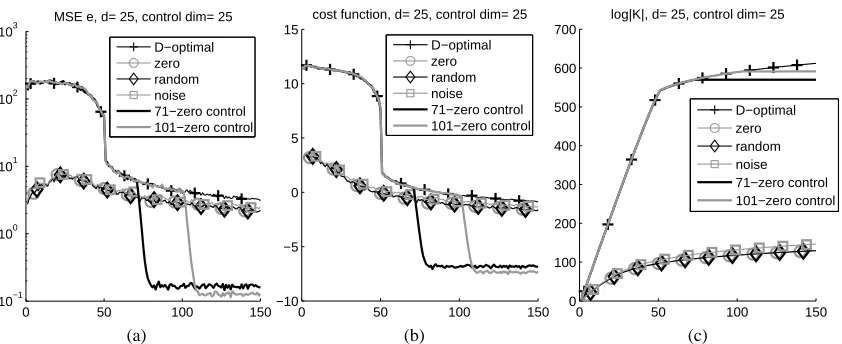
In the third experiment we used numerical tools to support our the arguments we made in Sec-tion 9. We investigate the D-optimal, the zero, the random, and the greedy noise control of (25), as

well as the 71-zero and 101-zero controls. Results show that if we may sacrifice the firstτsteps,

then the non-myopicτ₋zero control gives rise to the smallest MSE for the estimated noise and the

smallest values for the cost function (25) afterτsteps considering all studied control methods.

Fig-ure 5a shows the MSE of the estimated driving noise, whereas Fig. 5b depicts the cost xT_t₊₁K−_t 1xt+1.

Figure 5c is about the time dependence of log_|Kt|that supports our argument in Section 9, namely, it

may be worth to sacrifice steps at the beginning to quickly decrease_|K−t 1|(i.e., to decrease log|Kt|) in order to estimate (25) efficiently later. The problem we studied was the same as before, except

that d=25 and c=25 were applied.

The fourth experiment illustrates the efficiency of the approximation of the noise for the case

when our assumptions on etare not fulfilled. Here noise etwas neither Gaussian nor i.i.d. ‘Noise’ et

was chosen as equidistant points smoothly ‘walking’ along a 3 dimensional spiral curve as a function of time (Fig. 6a). Dimensions of observation and control were 3 and 15, respectively. Results are shown in Fig. 6. Neither random control, nor infomax interrogation of Table 1 (Fig. 6c), nor zero

(18)

0 50 100 150 200 10−4 10−2 100 102 104 106

MSE e, d= 10, control dim= 15

a b c d e f

a, 21−zero control b, 51− zero control c, 81− zero control d, 21−infomax noise e, 51−infomax noise f, 81−infomax noise

(a)

0 50 100 150 200

−15 −10 −5

0 cost fun, d= 10, control dim= 15

a

b _c d _e

f

a, 21−zero control b, 51−zero control c, 81−zero control d, 21−infomax noise e, 51−infomax noise f, 81−infomax noise

(b)

Figure 3: Comparing τ-infomax noise andτ-zero interrogations. The curves are averaged for 50

runs. Dimension of the control is 15 and the dimension of the observation is 10. (a): MSE of the

estimated noise (b): Cost function as given in (25). ‘τ-infomax noise’ (τ-zero) means that up to step

numberτstrategy of Table 1 applies and then the control of Eq. (29) is followed.

0 50 100 150 200

10−4 10−2 100 102 104 106

a

f g h e

d c

b

a, zero control b, infomax control c, random control d, 11−zero control e, 31−zero control f, 51−zero control g, 71−zero control h, 91−zero control

(a)

0 50 100 150 200

10−1 100 101 102 103

a b

c

d

e f

g h

a, zero control b, infomax control c, random control d, 11−zero control e, 31−zero control f, 51−zero control g, 71−zero control h, 91−zero control

(b)

Figure 4: Mean Square Error of the estimated noise for different control strategies. Magnitude of

MSE as a function of time is averaged for 20 runs. (a): Dimension of the control is 40. F_∈R40×40,

B_∈R40×10. (b): Dimension of the control is 10. F_∈R10×10, B_∈R10×40. ‘τ-zero’ means that up to

step numberτthe strategy illustrated in Table 1 was applied and then zero control followed.

produced a good approximation for large enoughτvalues (Fig. 6e). Details of this illustration are

shown in Fig. 6f.

10.1.3 JOINTPARAMETER ANDNOISEESTIMATIONS

(19)

0 50 100 150 10−1

100 101 102 103

D−optimal zero random noise 71−zero control 101−zero control

(a)

0 50 100 150

−10 −5 0 5 10 15

cost function, d= 25, control dim= 25

(b)

0 50 100 150

0 100 200 300 400 500 600 700

log|K|, d= 25, control dim= 25

(c)

Figure 5: Empirical study on non-myopic controls for noise estimation. We sacrifice the first τ

steps to achieve better MSE and smaller cost function. The curves are averaged over 25 runs. The dimension of the control and the dimension of the observation is 25. (a): MSE of noise estimation for different control strategies. (b): xT_t₊₁K−t 1xt+1cost function for different control strategies. (c):

log_|Kt|function for different control strategies.

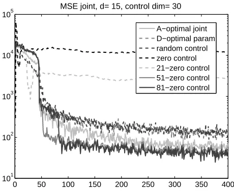
Studies were conducted on the problem family of 10.1.1 for observation dimension d=15 and

control dimension c=30. For the optimization, we modified the simplex method that we used for

the hyperbolic task before. The single difference is that upon convergence, the best value was com-pared with the value of the objective at the 0 point and we chose the better one for control. We have compared this strategy with the parameter estimation strategy of the D-optimality principle, with

zero control strategy, with random control strategy, and withτ₋zero control for severalτ values.

Results are shown in Fig. 8. The figure indicates that control derived from the A-optimality princi-ple (28) provides superior MSE results at approximately 45 iterations and then onwards compared to the other myopic techniques, however its performance was slightly worse than the non-myopic

τ-zero control forτvalues larger than an appropriate threshold.

Inspecting the optimal control series of the winner, we found that the algorithm chooses control values from the boundaries of the hypercube in the first 45 or so iterations. Then up to about 130 iterations it is switching between zero control and controls on the boundaries, but eventually it uses zero controls only. That is, the A-optimality principle is able to detect the need for the switch from high control values (to determine the parameters of the dynamics) to zero control values for noise estimation. This automated switching behavior is a special advantage of the A-optimality principle.

10.2 Controlled Independent Component Analysis

(20)

−1

0

1

−1 0 10 0.05 0.1 0.15 0.2

original noise

(a)

−1

0

1

−1 0 1 0 0.05 0.1 0.15 0.2

random control

(b)

−1

0

1

−1 0 10 0.05 0.1 0.15 0.2

infomax

(c)

−5 0

5 10

x 10−3 0.04

0.06 0.08 0.1 0.02 0.04 0.06 0.08

zero control

(d)

−1

0

1

−1 0 1 0 0.05 0.1 0.15 0.2

51−zero

(e)

0 50 100 150 200 10−4

10−2 100 102 104 106

zero control infomax control random control 21−zero control 51−zero control 81−zero control

(f)

(21)

(a) (b)

Figure 7: Negative logarithm of the objective function for the joint parameter and noise estimation task for different K matrices. (a) the minimum point is in zero, (b) the minimum point is on the boundary.

0 50 100 150 200 250 300 350 400 101

102 103 104 105

MSE joint, d= 15, control dim= 30

A−optimal joint D−optimal param random control zero control 21−zero control 51−zero control 81−zero control

Figure 8: MSE of the joint parameter and noise estimation task. Comparisons between joint param-eter and noise estimation using A-optimality principle, paramparam-eter estimation using D-optimality

principle, random control, zero control andτ₋zero control for differentτvalues. MSE values are

averaged for 20 experiments.

.

assume that the processes can be exogenously controlled. Such processes are called ARX processes where X stands for letter x of the word eXogenous.

The ‘classical’ ICA task is as follows: we are given temporally i.i.d. signals et ∈Rd (t=

1,2, . . . ,T)with statistically independent coordinates. We are unable to measure them directly, but

their mixture rt=Cet is available for observation, where C∈Rd×dis an unknown invertible matrix.

(22)

There are several generalizations of this problem. Hyvärinen (1998) has introduced an algorithm to solve the ICA task even if the hidden sources are AR processes, whereas Szabó and L˝orincz

(2008) generalized this problem for ARX processes in the following way: Processes ˜et ∈Rd are

given and they are statistically independent for the different coordinates and are temporally i.i.d signals. They generate ARX process st by means of parameters ˜F∈Rd×d,B˜ ∈Rd×c:

st+1=

I

∑

i=0

˜

Fist₋i+ J

∑

j=0

˜

Bjut+1₋j+˜et+1. (30)

We assume that ARX process st can not be observed directly, but its mixture

rt=Cst (31)

is observable, where mixing matrix C∈Rd×dis invertible, but unknown. Our task is to estimate the

original independent processes also called sources, noises or ‘causes’, that is, ˜et, the hidden process

st and mixing matrix C from observations rt. It is easy to see that (30) and (31) can be rewritten

into the following form

rt+1=

I

∑

i=0

C ˜FiC−1rt−i+ J

∑

j=0

C ˜But+1−j+C˜et+1. (32)

Using notations Fi=C ˜FiC−1, Bj=C ˜Bj, et+1=C˜et+1, (32) takes the form of the model (1) that we

are studying with function g being the identity matrix. The only difference is that in ICA tasks et is

assumed to be non-Gaussian, whereas in our derivations we always used the Gaussian assumption. In our studies, however, we found that the different control methods can be useful for non-Gaussian

noise, too. Furthermore, the Central Limit Theorem says that the mixture of the variables ˜et, that

is, C˜et approximates Gaussian distributions, provided that the number of mixed variables is large

enough.

In our numerical experiments we studied the following special case:

rt+1 = Frt+But+1+Cet+1,

where the dimension of the noise was 3, the dimension of the control was 15. Matrices F and B were generated the same way as before, matrix C was a randomly chosen orthogonal mixing, noise

sources et+1 were chosen from the benchmark tasks of the fastICA toolbox1 (Hyvärinen, 1999).

We compared 5 different control methods (zero control, D-optimal control developed for parameter estimation, random control, A-optimal control developed for joint estimation of parameters and

noise, as well as theτ-zero control withτ=81 that we developed for noise estimation). Comparisons

are executed by first estimating the noise (Cet+1) for times T =1, . . . ,1000 and then applying the

JADE ICA algorithm (Cardoso, 1999) for the estimation of the noise components (et+1). Estimation

was executed in each fiftieth steps, but only for the preceding 300 elements of the time series. The quality of separation is evaluated by means of the Amari-error (Amari et al., 1996) as

follows. Let W_∈Rd×d be the estimated demixing matrix, and let G :=WC_∈Rd×d. In case