ISSN 2466-4294 (online) | rad-journal.org Vol. 2 | Issue 3 | pp. 181 – 185, 2017 doi: 10.21175/RadJ.2017.03.037 Original research paper
CALCULATION OF THALLIUM HYPERFINE ANOMALY
*E. A. Konovalova1**, M. G. Kozlov1,2, Yu. A. Demidov1,2, A. E. Barzakh1
1Petersburg Nuclear Physics Institute, Gatchina, Russia
2St. Petersburg Electrotechnical University “LETI”, St. Petersburg, Russia
Abstract. We suggest a method of a computation of hyperfine anomaly for many-electron atoms and ions. At first, we tested this method by calculating the hyperfine anomaly for a hydrogen-like thallium ion and obtained fairly good agreement with analytical expressions. Then, we did calculations for the neutral thallium and tested an assumption that the ratio between the anomalies for s and p1/2 states is the same for these two systems. Finally, we come up with
recommendations about the preferable atomic states for the precise measurements of the nuclear g factors. Key words:Hyperfine anomaly, hyperfine structure, thallium, nuclear distribution, Bohr–Weisskopf effect
1.INTRODUCTION
In recent years, the precision achieved in resonant ionization spectroscopy experiments coupled with advances in atomic theory has enabled new atomic physics based tests of nuclear models. Understanding the occurrence of shape coexistence in atomic nuclei is one of them. This phenomenon is associated with the existence of both the near-spherical and deformed structures of nuclei for neutron-deficient isotopes near the value of Z = 82 closed shell [1]. The measurements of hyperfine constants and isotope shifts are highly sensitive to the changes of the nuclear charge and magnetic radii because they depend on the behavior of the electron wave function near the nucleus. The hyperfine structure (HFS) splitting measurements can serve as a very useful tool for the understanding of the shape coexistence phenomena in atomic nuclei.
Magnetic hyperfine constants A are usually assumed to be proportional to the nuclear magnetic moments. However, this is true only for the point-like nucleus. For the finite nucleus, we need to take into account (i) distribution of the magnetization inside the nucleus and (ii) dependence of the electron wave function on the nuclear charge radius. Former correction is called magnetic (Bohr–Weisskopf) [2] and the latter is called charge correction (Breit-Rosenthal) [3, 4]. Together, these corrections are known as the hyperfine anomaly [5]. Below, we discuss how to calculate the hyperfine anomaly for many-electron atoms with the available atomic packages. We use a thallium atom as a reference system for our calculations, because there are comprehensive experimental data [6-10] and many theoretical calculations for this atom [5, 11-14].
Shabaev [5] and Shabaev et al. [11] found the analytical expressions for the hyperfine anomaly for H-like thallium ion. For the neutral thallium, there is the numerical calculation by Mårtensson-Pendrill [12].
* The paper was presented at the Fifth International Conference on Radiation and Applications in Various Fields of Research
(RAD 2017), Budva, Montenegro, 2017.
Experimentally, HFS anomaly is studied much better for a neutral Tl than for a respective H-like ion. In the work [15], it has been suggested that the ratio between the anomalies for s and p1/2 states remains constant for
these two systems. Here we try to test this assumption. We use the atomic package [16], which is based on the original Dirac-Hartree-Fock code [17]. This package is often used to calculate different atomic properties including hyperfine structure constants of Tl [13,14], Yb [18], Mg [19], and Pb [20].
2.THEORY AND METHODS
A four component Dirac wave function of an electron in a spherically symmetric atomic potential can be written as [17]:
𝜓𝑛,𝜅,𝑚(𝒓) = 1 𝑟(
𝑃𝑛,𝜅(𝑟)Ω𝜅,𝑚(𝜔)
−𝑄𝑛,𝜅(𝑟)Ω−𝜅,𝑚(𝜔)), (1)
where the relativistic quantum number κ=(𝑙 − 𝑗)(2j + 1) and 𝛺κ,m is the spherical spinor. In these notations, the radial integral for the magnetic hyperfine constant for the point-like nuclear magnetic moment in the origin has the form:
𝐼𝑛′,𝜅′,𝑛,𝜅= ∫ (𝑃𝑛′,𝜅′ ∞
0 𝑄𝑛,𝜅+ 𝑄𝑛′,𝜅′𝑃𝑛,𝜅) 𝑑𝑟
𝑟2. (2)
In the case of uniformly distributed magnetic moment over the nucleus of radius 𝑅𝑁 the part of this radial integral inside the nucleus modifies to [12]:
𝐼𝑛′,𝜅′,𝑛,𝜅𝑛𝑢𝑐 = ∫ (𝑃 𝑛′,𝜅′ 𝑅𝑁
0 𝑄𝑛,𝜅+ 𝑄𝑛′,𝜅′𝑃𝑛,𝜅)
𝑟𝑑𝑟
𝑅𝑁3. (3)
Outside the nucleus we can still use the integrand from Eq. (2).
𝑃𝑛,𝜅(𝑟)|𝑟≤𝑅𝑁= 𝑟
|𝜅|∑ 𝑃 𝑛,𝜅,𝑘𝑥𝑘 𝑀
𝑘=0 , 𝑥 =
𝑟
𝑅𝑁. (4)
With the help of this expansion, we can calculate the integral (3):
𝐼𝑛𝑛𝑢𝑐′,𝜅′,𝑛,𝜅=
𝑅𝑁|𝜅
′|+|𝜅|−1
∑ ∑ 𝑃𝑛′,𝜅′,𝑘𝑄𝑛,𝜅,𝑚−𝑘+𝑄𝑛′,𝜅′,𝑘𝑃𝑛,𝜅,𝑚−𝑘
|𝜅′|+|𝜅|+𝑚+2
𝑚 𝑘=0 𝑀
𝑚=0 . (5)
Note that nuclear contribution to the integral (2) can be written as:
𝐼𝑛𝑛𝑢𝑐,0′,𝜅′,𝑛,𝜅=
𝑅𝑁|𝜅′|+|𝜅|−1∑ ∑ 𝑃𝑛′,𝜅′,𝑘𝑄𝑛,𝜅,𝑚−𝑘+𝑄𝑛′,𝜅′,𝑘𝑃𝑛,𝜅,𝑚−𝑘
|𝜅′|+|𝜅|+𝑚−1
𝑚 𝑘=0 𝑀
𝑚=0 . (6)
Using expression (6) for two different nuclear radii, we can calculate the charge correction to atomic HFS, while using the expression (5) we simultaneously account for the charge and magnetic corrections. However, these two models are not sufficiently flexible to accurately describe the hyperfine anomaly. Expressions (2) and (3) correspond to two variants of the distribution of the magnetic moment: either homogeneous distribution over the whole nucleus, or point-like dipole in the origin. Introducing the magnetic radius 𝑅𝑀, we get either𝑅𝑀 = R𝑁or 𝑅𝑀= 0. If we want to allow for the arbitrary value 𝑅𝑀≤ 𝑅𝑁, we need to combine the integrand from Eq. (3) for r < R𝑀 with the integrand from Eq. (2) for 𝑅𝑀≤ 𝑟 ≤ 𝑅𝑁. Then we can write the integral over the nucleus as
𝐼𝑛𝑛𝑢𝑐′,𝜅′,𝑛,𝜅(𝑅𝑁, 𝑅𝑀) = 𝐼𝑛𝑛𝑢𝑐′,𝜅′,𝑛,𝜅(𝑅𝑀) + (𝐼𝑛𝑛𝑢𝑐,0′,𝜅′,𝑛,𝜅(𝑅𝑁) −
𝐼𝑛𝑛𝑢𝑐,0′,𝜅′,𝑛,𝜅(𝑅𝑀)), (7)
𝐼𝑛𝑛𝑢𝑐′,𝜅′,𝑛,𝜅(𝑅𝑀) =
𝑅𝑀|𝜅′|+|𝜅|−1∑ ∑ 𝑃𝑛′,𝜅′,𝑘𝑄𝑛,𝜅,𝑚−𝑘+𝑄𝑛′,𝜅′,𝑘𝑃𝑛,𝜅,𝑚−𝑘
|𝜅′|+|𝜅|+𝑚+2
𝑚 𝑘=0 𝑀
𝑚=0 (
𝑅𝑀
𝑅𝑁)
𝑚
, (8)
𝐼𝑛𝑛𝑢𝑐,0′,𝜅′,𝑛,𝜅(𝑅𝑀) =
𝑅𝑀 |𝜅′|+|𝜅|−1
∑ ∑ 𝑃𝑛′,𝜅′,𝑘𝑄𝑛,𝜅,𝑚−𝑘+𝑄𝑛′,𝜅′,𝑘𝑃𝑛,𝜅,𝑚−𝑘
|𝜅′|+|𝜅|+𝑚−1
𝑚 𝑘=0 𝑀
𝑚=0 (
𝑅𝑀
𝑅𝑁)
𝑚
. (9)
2.1. Isotope effect for magnetic HFS
Suppose we want to compare hyperfine constants 𝐴1 and 𝐴2 for two isotopes with nuclear g factors 𝑔(1)𝐼 and 𝑔(2)
𝐼 (𝑔𝐼 = μ 𝐼⁄ ), nuclear charge radii 𝑅𝑁 (1) and
𝑅𝑁(2) , and magnetic radii 𝑅𝑀(1) and 𝑅𝑁(2). We can write:
𝐴1
𝐴2=
𝑔(1) 𝐼
𝑔(2) 𝐼
(1 − 𝜆𝐶 𝑅𝑁 (1)
−𝑅𝑁(2) 𝑅𝑁(1)+𝑅𝑁(2)− 𝜆
𝑀 𝑅𝑀 (1)
−𝑅𝑀(2)
𝑅𝑀(1)+𝑅𝑀(2)). (10) The anomaly then has the following form:
1Δ2≡𝑔(2)𝐼𝐴1
𝑔(1)
𝐼𝐴2− 1 = − (𝜆
𝐶 𝑅𝑁 (1)
−𝑅𝑁(2) 𝑅𝑁(1)+𝑅𝑁(2)+ 𝜆
𝑀 𝑅𝑀 (1)
−𝑅𝑀(2) 𝑅𝑀(1)+𝑅𝑀(2))(11) By solving above equations for several radii, we can find 𝜆𝐶 and 𝜆𝑀 and calculate the anomaly for the isotopes of interest. Below we will see that parameters 𝜆𝐶 and 𝜆𝑀 themselves depend on the radii 𝑅𝑁 and 𝑅𝑀. Therefore, it is better to use parameters 𝑏𝑁 and 𝑏𝑀 defined below (see Eq. (18)).
2.2. Hydrogen-like ions
It is generally accepted that the observed hyperfine constant 𝐴(𝑅𝑁,R𝑀)of a one-electron ion may be presented in the following form:
𝐴(𝑅𝑁,R𝑀)=A0(1 − 𝛿(𝑅𝑁))(1 − 𝜖(𝑅𝑀)). (12) Here 𝐴0≡ 𝐴(0,0) is the factor which is independent of the nuclear radii and 𝛿(𝑅𝑁) and𝜖(𝑅𝑀) are the nuclear charge distribution and magnetic distribution corrections respectively. For a given Z and electron state, they can be written as:
𝛿(𝑅𝑁)=b𝑁𝑅𝑁 (2𝛾−1),
𝜖(𝑅𝑁)=b𝑀𝑅𝑀
(2𝛾−1), (13) where 𝑏𝑁 and 𝑏𝑀are the factors which are independent of the nuclear radii, γ=√𝜅2+ (αZ)2, and 𝛼 is the fine structure constant. The expression for 𝐴0 was obtained in the analytical form as [5]:
𝐴0=
𝛼(αZ)3𝑔 𝐼
𝑗(j+1) 𝑚 𝑚𝑝
𝜅(2𝜅(γ+n𝑟)−𝑁) 𝑁4𝛾(4𝛾2−1) mc
2. (14)
Here,𝑚 and 𝑚𝑝are the electron and proton masses, 𝑔𝐼 is the nuclear g factor, j is the total electron angular momentum, N=√𝑛𝑟2+ 2n𝑟2𝛾 + 𝜅2, 𝑛𝑟 is the radial quantum number.
It follows from Eqs. (12) and (13) that if we calculate HFS constant numerically for different 𝑅𝑁 and 𝑅𝑀 , we should get the following dependence on the radii:
𝐴(𝑅𝑁,R𝑀)=A0(1 − 𝑏𝑁𝑅𝑁 2𝛾−1
)(1 − 𝑏𝑀𝑅𝑀 2𝛾−1
) (15) This expression defines the dependence of parameters 𝜆𝐶and 𝜆𝑀 from (10) on the radii 𝑅
𝑁and 𝑅𝑀. For example, on the one hand, we have:
𝐴(𝑅𝑁+ρ,R𝑀)
𝐴(𝑅𝑁−ρ,R𝑀)
= 1 − 𝜆𝐶(𝑅 𝑁)
𝜌 𝑅𝑁
. (16)
On the other hand: 𝐴(𝑅𝑁+ρ,R𝑀)
𝐴(𝑅𝑁−ρ,R𝑀)
= 1 + 2𝜌𝜕𝐴(𝑅𝑁,R𝑀) 𝜕𝑅⁄ 𝑁
𝐴(𝑅𝑁,R𝑀)
. (17)
Then, from Eq. (16) we get: 𝜆𝐶(𝑅
𝑁) ≈
2(2𝛾−1)𝑏𝑁𝑅𝑁 2𝛾−1
1−𝑏𝑁𝑅𝑁2𝛾−1
≈ 2(2𝛾 − 1)𝑏𝑁𝑅𝑁
2𝛾−1. (18)
Similar expressions can be obtained for 𝜆𝑀(𝑅 𝑀).For the point-like magnetic dipole approximation (𝑅𝑀= 0) the magnetic correction is equal to zero, and the hyperfine constant can be fitted by the function:
𝐴(𝑅𝑁, 0) = 𝐴0(1 − 𝑏𝑁𝑅𝑁
2𝛾−1
). (19)
For the uniform distribution of the charge and magnetic moment with the value of𝑅𝑀 = R𝑁 we get:
𝐴(𝑅𝑁, 𝑅𝑁) = 𝐴0(1 − (𝑏𝑁+ 𝑏𝑀)𝑅𝑁 2𝛾−1
). (20)
2.3. Many-electron atoms
can do configuration interaction calculations with the frozen core and few valence electrons. Then we can add the core-valence correlation corrections with the help of the many-body perturbation theory. At this stage, we substitute the valence radial integrals with the effective ones, which account for the spin polarization of the core. The latter are obtained by solving random-phase approximation (RPA) equations.
Effective radial integrals may have significantly different dependence on the parameters of the nucleus than initial “bare” integrals. This is particularly true for the orbitals with the high angular momentum. Because of the centrifugal barrier, these orbitals do not penetrate inside the nucleus and bare radial integrals do not depend on the nuclear size. On the other hand, spin-polarization of the core always includes spin-polarization of the core s andp1/2 shells. Because of that, all effective radial integrals are sensitive to the nuclear charge and magnetic distributions. In general, we can divide all correlation corrections in two classes: corrections, which mix orbitals within one partial wave, and the ones which mix different partial waves. For example, the self-energy type corrections belong to the first class. They mix core and valence orbitals of the same symmetry and can significantly change the orbital density at the origin. Therefore, these corrections change the size of the HFS matrix elements. On the other hand, all orbitals of the same symmetry have practically the same sensitivity to the nuclear distributions. Thus, such correlation corrections do not affect parameters 𝑏𝑁 and 𝑏𝑀 and the HFS anomaly (11). RPA corrections belong to the second class, which significantly contribute to the HFS anomaly.
Measurement of hyperfine anomaly for highly charged ions allows experimental study of QED effects (see e.g. [21]). Attempts to take into account QED corrections in hyperfine structure calculations for such systems have already been made [8, 22, 23]. However, for neutral atoms QED corrections are sufficiently small and should be taken into account only after correlation effects. It can be done using the method recently described in the article [24]. Note, that dominant QED corrections belong to the first class and do not significantly affect the HFS anomaly.
3.RESULTS AND DISCUSSION
3.1. HFS anomaly for H-like thallium ion
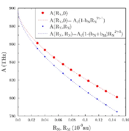
In this section, we calculate the HFS constants of the 1s, 2s, and 2p1/2 states of Tl80+ for different radii 𝑅𝑁 and 𝑅𝑀 and compare our results with the analytical expressions from Ref. [5]. Figure 1 shows the dependence of the hyperfine constant A(1s) on the radii 𝑅𝑁 and 𝑅𝑀. We see very good agreement with Eqs. (19) and (20).
Table I summarizes our results for H-like Tl ion. We see the perfect agreement of the calculated and analytical values of 𝐴0 for all three states. Charge and magnetic corrections δ and ε were calculated in Ref. [11] for the 1s state of the isotope 203Tl. These analytical
values are also in a good agreement with our numerical results.
Figure 1. The dependence of the HFS constant A(RN , RM) for
the ground state of H-like Tl ion from nuclear charge and magnetic radii. Dots and circles correspond to the computed
values. Dashed lines correspond to the fits by Eqs. (19) and (20).
Table 1. Compilation of the fitting parameters for HFS of H-like Tl ion: A0 is HFS constant for point-like nucleus, δ and ε
are the nuclear charge and magnetization distribution corrections parametrized by bN and bM coefficients
respectively. We use g factor gI = 3.27640. Corrections δ and ε
for 203Tl are calculated for RN = RM= 0.1306 × 10⁻³ au.
1s 2s 2p1/2
A0 (THz) fit. 896.4 144.9 45.0 Eq. (14) 895.7 144.8 45.0
bN fit. 0.3441 0.3671 0.0960
δ(203Tl80+) fit. 0.0988 0.1054 0.0276
Ref. [11] 0.0988 – –
bM fit. 0.0599 0.0638 0.0176
ε(203Tl80+) fit. 0.0172 0.0183 0.0051
Ref. [11] 0.0179 – –
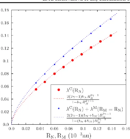
Figure 2 shows how parameters 𝜆 for the 1s state depend on the radii 𝑅𝑁 and 𝑅𝑀. We see the perfect agreement with the analytical expression (18). On the other hand, it means that these parameters strongly depend on the nuclear size. Because of that, they cannot be treated as a constant even for the isotopes with the similar radii. Therefore, it is better to use parameters 𝑏𝑁 and 𝑏𝑀 defined by Eq. (15).
According to our calculations (see Table I), the ratios of the parameters 𝑏𝑁 and 𝑏𝑀 for 1s and 2s states are close to unity: 𝑏𝑁(1𝑠)
𝑏𝑁(2𝑠)= 0.937 and
𝑏𝑀(1𝑠)
𝑏𝑀(2𝑠)= 0.939. This is
expected, as wave functions of the same symmetry should be proportional to each other inside the nucleus. Similar ratios for 1s and 2p1/2 states are 𝑏𝑁(1𝑠)
𝑏𝑁(2𝑝1 2⁄)= 3.58
and 𝑏𝑀(1𝑠)
𝑏𝑀(2𝑝1 2⁄)= 3.40. Again, one can expect that these
Figure 2. Dependence of the parameters λC(RN) and λM (RM)
(see Eq. (10)) on the charge and magnetic radii of the nucleus for the ground state of H-like Tl ion. Computed values represented by points. The curves correspond to the fits with
Eq. (18).
3.2. HFS anomaly of neutral thallium atom
The ground configuration of the neutral thallium is
[1s2 ... 6s2]6p and the ground multiplet includes two levels, 6p1/2 and 6p3/2. The lowest level of the opposite parity is 7s. Most of the experiments and calculations of the HFS in neutral thallium deal with these three levels. If we treat thallium as a one-electron system with the frozen core [1s2 ... 6s2], we can do the calculation using the Dirac-Hartree-Fock (DHF) method. In this case, the dependence of the HFS constants on the nuclear radii is similar to the one-electron ion.
In DHF approximation, the HFS constant with the value of A(6p3/2) = 1.30 GHz is very small and practically does not depend on 𝑅𝑁 and 𝑅𝑀 (see Table II). At the same time, the HFS constants A(6p1/2) and A(7s) are well described by Eqs. (19, 20) (see Fig. 3). According to our calculations, the ratios between the coefficients 𝑏𝑁 and 𝑏𝑀 for s and p1/2 waves are close to the respective ratios in the H-like ion. For example, the ratios of these constants for 1s state of the ion and 7s state of the neutral atom are 𝑏𝑁(1𝑠)
𝑏𝑁(7𝑠)= 0.926
and 𝑏𝑀(1𝑠)
𝑏𝑀(7𝑠)= 0.931
. Atomic ratios for 7s and 6p1/2 are: 𝑏𝑁(7𝑠)
𝑏𝑁(6𝑝1 2⁄)= 3.52 and
𝑏𝑀(7𝑠)
𝑏𝑀(6𝑝1 2⁄)= 3.30, while for the H-like ion we had the
values of 3.58 and 3.40 respectively.
Situation changes when we include the spin-polarization of the core via RPA corrections. These corrections mix partial waves and the state 6p3/2 partly
acquires and p1/2 character. This leads to the significant change of the size and even the sign of the constant
A(6p3/2). At the same time, this constant becomes very sensitive to the distributions of charge and magnetic moment inside the nucleus.
RPA corrections for the 7s and 6p1/2 states are smaller than for 6p3/2, but also significant. They lead to
effective mixing of the s and p waves. Because of that, the ratios of the respective coefficients decrease a little, but are still markedly larger than unity:
𝑏𝑁(7𝑠)
𝑏𝑁(6𝑝1 2⁄)= 2.65,
𝑏𝑀(7𝑠)
𝑏𝑀(6𝑝1 2⁄)= 2.44.
We conclude that in the DHF+RPA approximation, the anomaly for the 7s state is still significantly stronger, than for 6p1/2 state. The anomaly for the 6p3/2, on the contrary, becomes the largest. In this work we did not take into account more correlation corrections, but RPA contribution influences the anomaly more strongly than others and changes its behavior. When all corrections are taken into account our method usually gives an accuracy of few percent for neutral atoms, as it was done in [14].
Table 2. Compilation of the fitting parameters for HFS of neutral Tl atom: A0 is HFS constant for point-like nucleus, δ
and ε are the nuclear charge and magnetization distribution corrections parametrized by bN and bM coefficients
respectively. We use g factor gI = 3.27640. Corrections δ and ε
for 203Tl are calculated for RN = RM= 0.1306 × 10⁻³ au. Calculations are done within DHF and DHF+RPA
approximations.
DHF DHF+RPA
6p1/2 7s 6p3/2 6p1/2 7s 6p3/2
A0(GHz) 18.130 8.855 1.289 22.684 12.120 -2.4711
bN 0.1054 0.3708 0 0.1400 0.3714 0.5769
δ(203Tl) 0.0302 0.1064 0 0.0402 0.1066 0.1656
bM 0.0195 0.0643 0 0.0254 0.0619 0.0933
ε(203Tl) 0.0056 0.0185 0 0.0073 0.0178 0.0268
Using the experimentally measured value of the HFS anomaly (10) for the ground state 6p1/2 of the thallium two stable isotopes 205∆203(6p1/2) = −1.036(3) × 10−4 [6]
and the ratios (21) calculated here, we can obtain corresponding value for the 7s state within 𝑅𝑀=R𝑁 approximation: 205∆203(7s)= −2.6 × 10⁻⁴. This value is
significantly lower, than experimental value of−4.7(1.5)×10−4 obtained in Ref. [7].
4.CONCLUSIONS
via RPA corrections, only the hyperfine anomaly for the
7s state remains stable. The ratios between 7s and 6p1/2 states change by roughly 30%, and the anomaly for the
6p3/2 state becomes very large. We conclude that for the precision measurements of g factors it is preferable to use the hyperfine constants for s states, while the p3/2 states are least useful.
Acknowledgement: The paper is supported by RFBF
grant №17-02-00216 А.
REFERENCES
1. A. N. Andreyev et al., “A triplet of differently shaped spin-zero states in the atomic nucleus 186Pb,”Nature,
vol. 405, no. 6785, pp. 430 – 433, May 2000. DOI: 10.1038/35013012
PMid: 10839532
2. A. Bohr, V. F. Weisskopf, “The influence of nuclear structure on the hyperfine structure of heavy elements,”
Phys. Rev.,vol. 77, no. 1, pp. 94 – 98, Jan. 1950. DOI: 10.1103/PhysRev.77.94
3. J. E. Rosenthal, G. Breit, “The isotope shift in hyperfine structure,” Phys. Rev., vol. 41, no. 4, pp. 459 – 470, Aug. 1932.
DOI: 10.1103/PhysRev.41.459
4. M. F. Crawford, A. L. Schawlow, “Electron-nuclear potential fields from hyperfine structure,” Phys. Rev., vol. 76, no. 9, pp. 1310 – 1317, Nov. 1949.
DOI: 10.1103/PhysRev.76.1310
5. V. M. Shabaev, “Hyperfine structure of hydrogen-like ions,” J. Phys. B, vol. 27, no. 24, pp. 5825 – 5832, Dec. 1994.
DOI: 10.1088/0953-4075/27/24/006
6. A. Lurio, A. G. Prodell, “Hfs Separations and Hfs Anomalies in the 2P1/2 State of Ga69, Ga71, Tl203, and Tl205,”
Phys. Rev., vol. 101, no. 1, pp. 79 – 83, Jan. 1956. DOI: 10.1103/PhysRev.101.79
7. D. S. Richardson, R. N. Lyman, P. K. Majumder “Hyperfine splitting and isotope-shift measurements within the 378-nm 6P 1/2− 7S1/2 transition in 203Tl and 205Tl,” Phys. Rev. A, vol. 62, no. 1, 012510, Jul. 2000.
8. P. Beiersdorfer et al., “Hyperfine structure of hydrogenlike thallium isotopes,” Phys. Rev. A, vol. 64, no. 3, 032506, Sep. 2001.
DOI: 10.1103/PhysRevA.64.032506
9. P. Beiersdorfer et al., “Hyperfine structure of heavy hydrogen-like ions,” Nucl. Instr. Meth. Phys. Res. B, vol. 205, pp. 62 – 65, May 2003.
DOI: 10.1016/S0168-583X(03)00534-2
10. A. E. Barzakh et al., “Hyperfine structure anomaly and magnetic moments of neutron deficient Tl isomers with I= 9/2,” Phys. Rev. C, vol. 86, no. 1, 014311, Jul. 2012. DOI: 10.1103/PhysRevC.86.014311
11. V. M. Shabaev, M. Tomaselli, T. Kűhl, A. N. Artemyev and V. A. Yerokhin, “Ground-state hyperfine splitting of high-Z hydrogenlike ions,” Phys. Rev. A, vol. 56, no. 1, pp. 252 – 255, Jul. 1997.
DOI: 10.1103/PhysRevA.56.252
12. A.-M. Mårtensson-Pendrill, “Magnetic moment distributions in Tl nuclei,” Phys. Rev. Lett., vol. 74, no. 12, pp. 2184 – 2187, Mar. 1995.
DOI: 10.1103/PhysRevLett.74.2184 PMid: 10057864
13. V. A. Dzuba, V. V. Flambaum, M. G. Kozlov, S. G. Porsev, “Using effective operators in calculating the hyperfine structure of atoms,”J. Exp. Theor. Phys., vol. 87, no. 5, pp. 885 – 890, Nov. 1998.
DOI: 10.1134/1.558736
14. M. G. Kozlov, S. G. Porsev, W. R. Johnson, “Parity nonconservation in thallium,” Phys. Rev. A, vol. 64, no. 5, 052107, Nov. 2001.
DOI: 10.1103/PhysRevA.64.052107
15. M. G. H. Gustavsson, C. Forssen, A.-M. Må rtensson-Pendrill, “Thallium hyperfine anomaly,” Hyperfine Interact., vol. 127, no. 1-4, pp. 347 – 352, Aug. 2000. DOI: 10.1023/A:1012693012231
16. M. Kozlov, S. Porsev, M. Safronova, I. Tupitsyn, “CI -MBPT: A package of programs for relativistic atomic calculations based on a method combining configuration interaction and many-body perturbation theory,”
Comput. Phys. Commun., vol. 195, pp. 199 – 213, Oct. 2015.
DOI: 10.1016/j.cpc.2015.05.007
17. V. F. Bratsev, G. B. Deyneka and I. I. Tupitsyn, “Application of Hartree-Fock method to calculation of relativistic atomic wave functions,” Bull. Acad. Sci. USSR, Phys. Ser., vol. 41, p. 173, 1977.
18. S. G. Porsev, Y. G. Rakhlina, M. G. Kozlov, “Calculation of hyperfine structure constants for ytterbium,” J. Phys. B, vol. 32, no. 5, 1113, Mar. 1999.
DOI: 10.1088/0953-4075/32/5/006
19. N. K. Kjøller, S. G. Porsev, P. G. Westergaard, N. Andersen and J. W. Thomsen, “Hyperfine structure of the (3s 3d) 3DJ manifold of 25 Mg I,” Phys. Rev. A, vol. 91,
no. 3, 032515, Mar. 2015.
DOI: 10.1103/PhysRevA.91.032515
20. S. G. Porsev, M. G. Kozlov, M. S. Safronova and I. I. Tupitsyn, “Development of the configuration -interaction + all-order method and application to the parity-nonconserving amplitude and other properties of Pb,” Phys. Rev. A, vol. 93, no. 1, 012501, Jan. 2016. DOI: 10.1103/PhysRevA.93.012501
21. I. Klaft et al., “Precision Laser Spectroscopy of the Ground State Hyperfine Splitting of Hydrogenlike
209Bi82+,”Phys. Rev. Lett., vol. 73, no. 18, pp. 2425 –
2427, Oct. 1994.
DOI: 10.1103/PhysRevLett.73.2425 PMid: 10057056
22. A. V. Glushkov et al., “QED calculation of the superheavy elements ions: Energy levels, Lamb shift, hyperfine structure, nuclear finite size effect,” Nucl. Phys. A., vol. 734, suppl. 5, pp. E21 – E24, Apr. 2004.
DOI: 10.1016/j.nuclphysa.2004.03.010
23. O. Yu. Khetselius, “Relativistic perturbation theory calculation of the hyperfine structure parameters for some heavy-element isotopes,” Int. J. Quant. Chem., vol. 109, no. 14, pp. 3330 – 3335, Nov. 2009.
DOI: 10.1002/qua.22269
24. I. I. Tupitsyn, M. G. Kozlov, M. S. Safronova, V. M. Shabaev, V. A. Dzuba, “Quantum Electrodynamical Shifts in Multivalent Heavy Ions,”