A New 4th Order Hybrid Runge-Kutta Methods for Solving Initial Value Problems (IVPs)

(1)

http://www.sciencepublishinggroup.com/j/pamj doi: 10.11648/j.pamj.20180706.11

ISSN: 2326-9790 (Print); ISSN: 2326-9812 (Online)

A New 4

th

Order Hybrid Runge-Kutta Methods for Solving

Initial Value Problems (IVPs)

Bazuaye Frank Etin-Osa

Department of Mathematics and Statistics, University of Port Harcourt, Port Harcourt, Nigeria

Email address:

To cite this article:

Bazuaye Frank Etin-Osa. A New 4th Order Hybrid Runge-Kutta Methods for Solving Initial Value Problems (IVPs). Pure and Applied Mathematics Journal. Vol. 7, No. 6, 2018, pp. 78-87. doi: 10.11648/j.pamj.20180706.11

Received: November 13, 2018; Accepted: December 4, 2018; Published: January 2, 2019

Abstract:

Recently, there has been a great deal of interest in the formulation of Runge-Kutta methods based on averages other than the conventional Arithmetic Mean for the numerical solution of Ordinary differential equations. In this paper, a new 4th Order Hybrid Runge-Kutta method based on linear combination of Arithmetic mean, Geometric mean and the Harmonic mean to solve first order initial value problems (IVPs) in ordinary differential equations (ODEs) is presented. Also the stability region for the method is shown. Moreover, the new method is compared with Runge-Kutta method based on arithmetic mean, geometric mean and harmonic mean. The numerical results indicate that the performance of the new method show superiority in terms of accuracy to some of other well known methods in literature and the stability investigation is in agreement with the known fourth order Runge-Kutta methods but with excellent stability region.

Keywords:

Hybrid Methods, Stability, Mean

1. Introduction

It is well known that most of the Initial Value Problems (IVPs) are solved by Runge-Kutta methods which in turn being applied to compute numerical solutions for variety of problems that are modeled as the differential equations and their systems Runge-Kutta algorithms are used to solve differential equations efficiently that are equivalent to approximate the exact solutions.

Many schemes have been developed for the solution of initial value problems. According to Butcher [1], a number of different approaches have been used in the analysis of Runge-Kutta methods. This is where the proposed approach and method of analysis of order 4 R-K such as Dingwen and Tingting [2] that investigated A Fourth-order Singly Diagonally Implicit Runge-Kutta Method for Solving One-dimensional Burgers’ Equation becomes very relevant.

In the last few years, there has been a growing interest in problem solving systems based on the Runge-Kutta methods. Several methods have been developed using the idea of different means such as the geometric mean, centroidal mean, harmonic mean, contra-harmonic mean and the heronian mean. Wusueta [3] and Wusu and Akanbi [4], presented a three stage method based on the harmonic mean and a

multi-derivative method using the usual arithmetic mean respectively. Akanbi [5] developed a third-order method based on the geometric mean. But [6] and [7] introduced the concept of the heronian mean Evans and Yaacob [8] introduced a fourth-order method based on the harmonic mean while Yaacob and Sangui [9]also developed a fourth-order method which is an embedded method based on the arithmetic and harmonic mean. Wazwaz [10] showed comparison of modified Runge-Kutta methods based on varieties of means.

(2)

usual arithmetic averages in standard Runge-Kutta schemes. Ghazala and Amand [16] provided a Solution to fourth order three-point boundary value problem using ADM and RKM. In the paper, the authors developed a computational method for solving linear and nonlinear fourth order three-point boundary value problem (BVP).

It is pertinent to mention that no effort, so far, has been made to develop a 4th Order Runge-kutta Method based on a linear combination of arithmetic mean, the Harmonic mean and the Geometric mean. Keeping this in view, a modest effort has been made in the present paper to develop such a new efficient numerical algorithm which is, for the first time added to the literature. It is observed that the presently developed algorithm has also been found to be more suitable one to solve the system of ODEs. The stability analysis is also discussed.

Initial value problems (IVPs) such as

0 0

( ) ( , ( )), ( )

u x′ = f x u x u x = u (1)

is often used in our daily life during Mathematical modeling. Wherexis the independent variable which may indicate the time in a physical problem and the dependent variable

( )

u x is the solution. Moreover, since u x( )could be a N-dimensional vector valued function, the domain and range of the differential equation f and the solution u_{are given by}

:

: N

f

u



ℜ×ℜ → ℜ

  

ℜ → ℜ 

(2)

The above equation (1) where f is a function of both x and u _{which is called "non-autonomous". However, by} simply introducing an extra variable which is always exactly equal to x, it can easily be rewritten in an equivalent "autonomous" form below, where f is a function ofu_only:

( ) ( ( ))

u x′ = f u x (3)

Though several problems are naturally expressed in the non-autonomous form, the autonomous form of differential equation (3) is preferred for most of the theoretical investigations. In addition, the autonomous form has some merits in numerical analysis since it yields a greater possibility that numerical methods can solve the differential equation exactly. It is of interest to note that the differential equation by itself is not enough to give a unique solution. Hence, some other additional information is needed. However, if all components ofu_{are given at a certain value} of x, that is, "initial conditions", then the differential equation is called an "initial value problem (IVP)" which is closely and naturally involved with physical modeling.

2. Materials and Methods

The New 4th Order Runge-Kutta Method is derived out of the existing 4th Order classical RungeKutta Method which is

based on the conventional Arithmetic mean.

The general P-stage Runge-Kutta method for solving an IVP with the initial conditionu x( 0)=u0is defined from the well known numerical integrator as

1 ( , ; )

n n n n

u₊ =u +h

ϕ

x u h

Where

1

( , ; )

p

n n i i

i

x u h c w

ϕ

=

∑

With

1

( , )

i

i n i n ij j

j

w f x c h u a w

−

=

= + +

∑

(4)

The fourth order Runge-kutta Method to solve the IVP (1) is defined as

1 ( 1 2 2 2 3 4)

6

n n

h

u₊ =u + w + w + w +w (5)

Where

1 ( n, n) n

w = f x u = f (6)

2 ( , 1)

2 2

n n

h h

w = f x + u + w (7)

3 ( , 2)

2 2

n n

h h

w = f x + u + w (8)

4 ( n , n 3)

w = f x +h u +hw (9)

(5) can be written in the form

2 3 3 4

1 2

1

3 2 2 2

n n

w w w w

w w

h

u ₊ =u +  + + + + + 

  (10)

Equation (10) is known as Runge-kutta method based on arithmetic mean. This can be modified into a geometric mean as

(

)

1 1 2 2 3 3 4

3

n n

h

u ₊ =u + w w + w w + w w (11)

Also, Wazwaz [10] modifies the formula by replacing an arithmetic mean with harmonic mean, that is

2 3 3 4

1 2 1

1 2 2 3 3 4

n n

w w w w

w w

u u h

w w w w w w

+

 

= +  + + 

+ + +

  (12)

With w w1, 2,w and w3 4 defined as in (6), (7), (8) and (9) respectively.

(3)

arithmetic mean (AM), harmonic mean (HM)and geometric mean (GM) as introduced by Khattri [17] as follows

1 1 1 1 1 1

1 1

14 ( , ) ( , ) 32 ( , ) ( , )

45

RKM

AM w w HM w w GM w w

w w

ϕ = − + (13)

Considering the problem (1) and replacing the arithmetic mean in (12) by (13), yields

(

)

(

)

2 3 3 4

1 2

1 2 3 4

1 2 2 3 3 4

1

1 2 2 3 3 4

3 3

3

7 2 2

135 48

n n

w w w w

w w

w w w w

w w w w w w

h

u u

w w w w w w

+

   

+ + + − + + +

   

+ + +

   

 

= + _ _

 ₊ ₊ ₊ ₊ ₊ 

 

 

(14)

1

2 2 2 1

3 3 31 1 32 2

4 4 41 1 42 2 43 3

( , )

( , ( ))

n n n

n n

w f x u f

w f x ha u ha w

w f x ha u h b w b w

w f x ha u h b w b w b w

= = 

  

= + +

  

= + + + _

 

= + + + + 

(15)

With 1

2 1

2 21,

t

t t

t

a b

a b etc

−

=

∴ =

∑

Expanding w w1, 2,w and w3 4 via taylor series yields

1 ( n, n)

w = f x u = f

2 2 2 3 3 3 4 4 4

2 1 1 1 1

1 1 1

2 6 24

u uu uuu uuu

w = +f ha ff + h a f f + h a f f + h a f f (16)

Similarly, w3 is expanded as

{

}

3 2

2 2 2 3 2 2 2

3 2 3 1 3 1 3 1 2 1 2 3 1 2 3

3

3 3

2 3

( ) 2( ) ( )

2 2

( )

6

u u u uu uu

uuu

h h

w f h a a ff h a a ff a a a a a a a f f f a a f f

h

a a f f

= + + + + + + + +

+ +

(17)

Also, w4 is expanded as

{

2

2 2 2 2

4 4 5 6 1 5 6 2 3 4 5 6

3

3 3 2 2 2

1 3 6 1 5 6 2 3 1 5 6 2 3 4 5 6

3

3 3

4 5 6

( ) ( ) ( )

2

( ( ) 2( ( ))( ))

2

( )

6

u u uu

u u uu

uuu

h

w f h a a a ff h a a a a a ff a a a f f

h

h a a a ff a a a a a a a a a a a a a f f f

h

a a a f f

= + + + + + + + + +

+ + + + + + + + +

+ + +

(18)

(4)

1 4 5 6

135

n n

h

u₊ =u + p −p +p 

Where

(

)

4 1 2 3 4

2 3 3 4

1 2 5

1 2 2 3 3 4

6 1 2 2 3 3 4

7( 2 2 )

3 3

3

48

p w w w w

w w w w

w w p

w w w w w w

p w w w w w w

= + + +

 

= + + 

+ + +

 

= + +

2 2 2 3 3 3

4 1 1 1 2 3

2 2 3 2 3 2 2 2 2

1 3 1 3 1 2 1 2 3 2 3

3 3 3 2 3

2 3 4 5 6 1 5 6 2 3

2

2 2

4 5 6

7

42 14 7 14 ( )

3

14 7 ( 2( ) 2 ) 7 ( )

7

( ) 7 ( ) 7( ) 7 ( ( )

3

7

( )

2

u uu uuu u

u u uu uu

uuu u u

u

p f ha ff h a f f h a f f h a a ff

h a a ff h a a a a a a a f f f h a a f f

h a a f f h a a a ff a a h a a a f

h

a a a f f

= + + + + +

+ + + + + +

+ + + + + + + + +

+ + 3 3 3 2 2

1 3 6 1 5 6 2 3 1 5

2 3 3 3

6 2 3 4 5 6 4 5 6

7

7 ( ) 2

2

7

2( ( )) ( ) ( )

6

u u

u uu uuu

h a a a f h a a a a a a a

a a a a a a f f f h a a a f f

+ + + + + +

+ + + + + + +

To compute the Geometric mean part(p6), and applying a binomial expansion strategy with fractional index.

2 3

1 1 2 1

(1 1 ...

2 8 16

x x x x

+ = + + + + (19)

Applying (19) by setting 12

1 2 (1 ) , , (1)4

w w = f +x ∀i i

Evaluating w w1 2 in line with (19), yields

(

2 3

2 2 3 3

1

1 2 ₂ 1 1 1 1 1 1 1

2 3

2 2 2 2 3 2 2 2 2 3 3 3 3 4

1

1 1 1 1 1 1 1 1 1 1 1

4

2 3

2 2 3 3

1

1 1 1 1 1 1 1

2

1

1 ) 1

2 2 6

1

8 ₂ ₎

3

2

( ) 1

2 6

u uu uuu

u uu u u uu uuu

u uu uuu

w h h

w w w ha w f a w f a w f

f

w h

w ha w f h a w f h a w f h a w f f a w f

f

w h h

w ha w f a w f a w f

f



 

  _

= +  + + + − +

 

 



    

+ + + + + −

   

+ + + + 

 

            

(5)

(

3 2 3

3 3 2 2 3 2 2 4 3 4

1

1 1 1 1 1 1 1 1 1

6

3 3

2 2 2 2 2 2 2 2 2 3 3 3 2 4

1

1 1 1 1 1 1 1 1 1 1 1

4

2 3

2 2 3 3

1

1 1 1 1 1 1 1

2

3

3 3 )

2 2

1

( 2 )

16 3

2

( ) 1

2 6

u u uu u uu

u uu u u uu uuu

u uu uuu

w h h

w ha w f h a w f a w f a w f f

f

w h

w ha w f h a w f h a w f h a w f f a w f

f

w h h

w ha w f a w f a w f

f  + + + + +      + + + + + + +     + + + −                (20)

Substituting w1= f and simplifying we have

2 3 2 3 3

2 3 2 2 2 3 3 3

1 2 1 1 1 1 1 1 1

2 u 4 uu 4 uuu 8 u 8 u uu 16 u

h h h h h h

w w = + a f + a ff + a f f − a f − a ff f + a f (21)

In a similar way, w w2 3 and w w3 4 are evaluated as

(

)

(

)

(

)

2

2 2

2 3 1 2 3 1 3 1 2 3 1 2 3

2 2 2 2

2 3

1 3 1 3 1 2 3 1 2 3 1 2 3

2 2

1 2 3 ₃ ₃

2 3 1

2

3 3

1 3 1 2 3

3 2 2

2 3 1

1 ( ) 8 4 ( ) 2 ( )

2 16

4 4( ) 4 ( ) 4 ( )

( )

4 32 4( ) 4

4 ( ( ) ) 12 16 u u uu u uu uuu h h

w w a a a f a a a a a a a a f

a a a a a a a a a a a a a

h h

a a a ff

a a a ff f

a a a a a

h h

a a a f f

= + + + + + + − + +  ₊ ₊ ₋ ₊ ₊ ₊ ₋   + + + _ _ + −   − + + + + 2 2

1 2 3 3

3 3

1 3 2 3 2 3 1

) ( )

4 ( ) ( ) u

a a a

f

a a a a a a a

 ₋ ₊ ₊    ₊ ₊ ₊ ₋    (22)

(

)

(

)

3 4 1 3 4 5 6

2

2 2

1 3 1 5 6 2 3 4 5 6 2 3 4 5 6 2 3

2

1 3 6 6 1 3 1 3 2 3

3

1 3 4 5 6 2 3 4 5 6

2 3

2 2

2 3 4 5 6

1 ( ) ( )

2

4( ) 4 ( ) 4( )(( ) ( ) ( ) )

8

8 4 ( ) 4 ( )

4 ( ) ( ) (

( ) ( ) 4 16 u u uu h

w w a a a a a f

h

a a a a a a a a a a a a a a a a a f

a a a a a a a a a a

a a a a a a a a a a

h h

a a a a a ff

= + + + + + + + + + + + + + − + + − + + + + + + + + + + + + + + + + + + +

(

)

3 3

1 5 4 5 6 1 2 3

2

6 2 3 4 5 6 2 3 4 5 6

2

2 3 4 5 6

3 2

1 3 1 5 1 3 2 3

2

1 5 4 5 6 6 2 3

3 3

2 3 2

4 5 6 2 3

)

4 ( ) 4 ( )

4 ( )( ) ( )( )

( ) ( )

2 2 4 ( )

4 ( ) 2 ( )

( ) ( )

12 8

u

uuu

a a a a a a a a f

a a a a a a a a a a a

a a a a a

a a a a a a a a

a a a a a a a a

h h

a a a a a f f

        + + + − +   ₋ ₊ ₊ ₊ ₋ ₊ ₊ ₊    ₋ ₊ ₊ ₊    + + + + + + + + + +

+ + + + + + 6 2 3 4 5 6

2

2 3 4 5 6

2 3

2 3 4 5 6 2 3

3

4 5 6

4 ( )( )

( )( )

( ) ( ) ( )

( )

a a a a a a

a a a a a

a a a a a a a

a a a

        + + + +    ₊ _{+ +} ₊     ₊ ₊ ₊ ₋ ₊    ₋ ₊ ₊    (23)

(6)

2

1 3 2 1

2 2 2 2 2 2

3 1 2

2 2 2

2 3 1 2 1 3

2 2 2 2 2 2 2 3

2 3 3 2 1

2 16 16 16

( )

5 100 100 50

16 16 16

( )

200 100 200

16 16 16

)

300 300 75

16 16 16 16

)

100 300 75 75

n n u u u

uu uu uu

u u u

uu u u u

h

u u f h a ff a ff a ff

a f f a f f a f f

a a ff a a f a a ff

a a f f a ff a ff a ff h

+ = + + + +

+ +

− + +

− − −

(24)

By setting ( ₂ ₃) 1, ( ₄ ₅ ₆) 1 2

a +a = a + +a a = and comparing (24) with the fourth order taylorseries expansion for y x( n+1),we

have the following six systems of equations

2

1

3 2 2

6 1 1 5 1 3 1

3 2 2

1

4 3 2

6 1 1 5 1 3 6 1

2 3

1 3 1

4 2 2

6 1 1 5 1 3 1

2 3

1 3 1

: 43 21 0

: 24 11 5 21 43 11 0

: 53 213 0

: 40 266 6 53 210 13

106 53 0

: 240 130 13 213 213 26

106 2106 0

a

u

uu

u

u uu

h ff a

h ff a a a a a a a

h f f a

h ff a a a a a a a a

a a a

h f f f a a a a a a a

a a a

− + =

− − − − + =

− =

+ + + − +

− − =

− − − − −

− + =

4 3 3

1

nd

: 88 711 0

uuu

h f f a

                     

− = 

(25)

Solving the above equations simultaneously, the six parameters values are to be determined. It is to be noticed that for simplicity, the algebra function f is considered as a function of u only

1 2 1 4 5 6

1 1 9 1 5 11

, , , , ,

4 32 32 16 48 24

a = a = − a = a = − a = a = (26)

With

1

2 1

3 1 2

4 1 2 3

( , ),

( , )

4 4

( , ( 9 )

4 32

( , ( 6 10 44 )

96

n n

w f x u

h h

w f x u w

h h

w f x u w w

h

w f x h u w w w

 

=

  

= + + 

   

= + + − +

   

= + + − + + _

(27)

3. Results

In this section we discuss the stability regions for the New 4th Order Runge-Kutta method based on a linear

combination of the Arithmetic mean, Geometric mean and the harmonic mean

(7)

approach shall be applied to establish the stability of this new scheme

The stability region largely depends on the initial value problem (IVP). According to Fatunla [19] and Lawson [20],

it should be noted that the condition n 1 1 n u

u + _<

must be

satisfied in order to determine the stability region of the New 4th Order Runge-Kutta method formula in the complex plane. With the help of stability polynomials, the stability regions for New 4th Order Runge-Kutta method based on a linear combination of the Arithmetic mean, Geometric mean and the harmonic mean can be obtained

To get the area or region, the differential equation y′ =

λ

y

can be evaluated by using y′ =

λ

y as a test of the equation. Substituting y′ into (27), we obtain

1

2 2

2 2 2 3

3

2 2 3 3 4

4

1 4

1 9

4 128

11 65

24 236

w y

w y h y

w y h y h y

w y h y h y h y

λ

λ λ

λ λ λ

λ λ λ λ

 

=

  

= + 

   

= + +

   

= + + + _

(28)

Substituting (28) into (14), letting z=h

λ

and applying binomial and geometric series, we obtain

2 3 4 5

1 ₁ 1 1 1 1

2 6 162 3645

n

y

z z z z z

y

+ _{= + +} ₊ ₊ _{+ +}

(29)

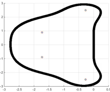
Using MATLAB package, we obtain the following results for the stability region for the new method

Figure 1. Stability Region of the new scheme.

The figure 1 above shows the stability region of the new method that is the set of complex values of h

λ

for which all solutions ofy′ =

λ

ywill remain bounded as n→ ∞

4. Discussion

In this section, the efficiency and suitability of the new computational methods is illustrated and discussed. The

(8)

figure 4).

Problem 1. u 1 u(0) 1 u

′ = = and the exact solution is

1 2

(2 1) [0,1]

u= x+ on

The results of problem 1 with different values of step sizes are presented in the figures below

Figure 2. The graph of RKAM and BAZM.

From the Figure 2 above, it is very clear that the propose method (BAZM) performs better in terms of accuracy than the Runge –Kutta method based on the Arithmetic Mean (RKAM).

Figure 3. The graph of RKMC and BAZM.

Again, BAZM clearly shows superiority over the RKMC From the graph above, it can be shown that the new method competes favorably with other existing methods in terms of accuracy.

Figure 4. The graph of RKMC. RKGM, RKHM and BAZM.

From the graph above, it can be shown that the new method competes favorably with other existing methods in terms of accuracy.

Figure 5. The graph of RKAM, RKMC, RKGM, BAZM and RKHAM.

Problem 2. 1 ₂ 2 2 (0) 0

1

u u u

x

′ = − =

+ and exact solution is

2

1

[0,1] 1

u on

x =

+

(9)

Figure 6. The graph of RKMC, RKGM, BAZM and RKHAM.

From the graph above, it can be shown that the new method competes favorably with other existing methods in terms of accuracy for problem 2.

From the graph above, it can be shown that the new method competes favorably with other existing methods in terms of accuracy for problem 2

Problem 3:

2_{(ln )}3 ₂ _{(ln )}4 _{2 ln} _2, ₍₁₎ ₀

u′ =u x − xu x + x+ u = and exact

solution isu=2 lnx x on[1, 2].

The results of problem 3 with different values of step sizes is represented in figure 4 below

5. Conclusion

In this paper, the derivation of the new hybrid 4th order Runge-kutta methods which are based on a linear combination of arithmetic mean, harmonic mean and the geometric mean have been successfully carried out. Also, the region of stability was established with the aid of a MATLAB by drawing the curve of stability polynomial. It is revealed that the stability region of the new method is the set of complex values of h

λ

for which all solutions ofy′ =

λ

ywill remain bounded asn→ ∞_. Several practically applicable problems have been considered to test the suitability, adoptability and accuracy of the proposed method. To achieve this, three test problems were considered and the results indicate that the New method is stable and of high degree of accuracy in comparison with the other existing methods.

References

[1] J. C Butcher (1987). The Numerical Analysis of Ordinary Differential equations. Runge-kutta and Genaral Linear Methods. Wiley international science publications. Printed and bound in the Great Britain.

[2] D. Dingwen and P. Tingting (2015). A Fourth-order Singly Diagonally Implicit Runge-Kutta Method for Solving One-dimensional Burgers’ Equation. IAENG International Journal of Applied Mathematics, 45, 4-11.

[3] A. S Wusu, S. A Okunuga, A. B Sofoluwe (2012). A Third-Order Harmonic explicit Runge-Kutta Method for Autonomous initial value problems. Global Journal of Pure and Applied Mathematics. 8, 441-451.

(10)

[5] M. AAkanbi (2011). On 3- stage Geometric Explicit Runge-Kutta Method for singular Autonomous initial value problems in ordinary differential equations computing. 92, 243-263. [6] J. D Evans and N. B Yaacob (1995). A Fourth Order Runge –

Kutta Methods based on Heronian Mean Formula. International Journal of Computer Mathematics 58, 103-115. [7] J. D Evans and N. B Yaacob (1995) A Fourth Order Runge –

Kutta Methods based on Heronian Mean Formula. International Journal of Computer Mathematics 59, 1-2. [8] J. D Evans and N. B Yaacob (1995). A New Fourth Order

Runge –Kutta Methods based on Heronian Mean Formula. Department of Computer studies, Loughborough University of technology, Loughborough.

[9] N. B Yaacob and B. Sangui (1998). A New Fourth Order Embedded Method based on Heronian Mean Mathematica Jilid, 1998, 1-6.

[10] A. M. Wazwaz (1990). A Modified Third order Runge-kutta Method. Applied Mathematics Letter, 3(1990), 123-125. [11] J. D Evans and B. Sangui(1991). AComparison of Numerical

O. D. E solvers based on Arithmetic and Geometric means. International Journal of Computer Mthematics, 32-35. [12] S. O. Fatunla (1988). Numerical Methods for initial value

problems in ordinary Differential equations Academic Press, San Diago.

[13] G. U, Agbeboh, U. S. U Aashikpelokhai., I. Aigbedion.

(2007). Implementation of a New 4th order RungeKutta Formula for solving initial value problems International Journal of Physical Siences. 2(4), 89-98.

[14] Y Rini. Imran M, Syamsudhuha. A Third RungeKutta Method based on a LAinear combination of Arithmetic mean, harmonic mean and geometric mean. Applied and Computational Mathematics. 2014, 3(5), 231-234.

[15] Ashirobo Serapon (2015). On the Derivation and Implementation of a Four Stage Harmonic ExplicitRunge-Kutta Method Ashirobo serapon. Applied Mathematics 6(4):694-699.

[16] A. Ghazala and I. Ahmand, (2016). Solution of fourth order three-point boundary value problem using ADM and RKM. Journal of the Association of Arab Universities for Basic and Applied Sciences. 20, 61-67.

[17] S. K. Khattri (2012). Eulers Number and some Means. Tamsui Oxford Journal of Information and Mathematical Sciences28 (2012), 369-377.

[18] G. U. Agbeboh (2013). On the Stability Analysis of a 4th order Runge- kutta method based onGeometric mean. Mathematical Theory and Modeling, 4, 76-91.

[19] S. O. Fatunla (1986). Numerical Treatment of singular IVPs. Computational Math. Application. 12:1109-1115.