Global Analytic Solution of Fully-observed Variational Bayesian Matrix Factorization

Global Analytic Solution of Fully-observed Variational Bayesian

Matrix Factorization

∗

Shinichi Nakajima NAKAJIMA.S@NIKON.CO.JP

Optical Research Laboratory Nikon Corporation

Tokyo 140-8601, Japan

Masashi Sugiyama SUGI@CS.TITECH.AC.JP

Department of Computer Science Tokyo Institute of Technology Tokyo 152-8552, Japan

S. Derin Babacan DBABACAN@ILLINOIS.EDU

Beckman Institute

University of Illinois at Urbana-Champaign Urbana, IL 61801 USA

Ryota Tomioka TOMIOKA@MIST.I.U-TOKYO.AC.JP

Department of Mathematical Informatics The University of Tokyo

Tokyo 113-8656, Japan

Editor:Manfred Opper

Abstract

The variational Bayesian (VB) approximation is known to be a promising approach to Bayesian estimation, when the rigorous calculation of the Bayes posterior is intractable. The VB approxima-tion has been successfully applied tomatrix factorization(MF), offering automatic dimensionality selection for principal component analysis. Generally, finding the VB solution is a non-convex problem, and most methods rely on a local search algorithm derived through a standard procedure for the VB approximation. In this paper, we show that a better option is available for fully-observed VBMF—the global solution can beanalyticallycomputed. More specifically, the global solution is a reweighted SVD of the observed matrix, and each weight can be obtained by solving a quartic equation with its coefficients being functions of the observed singular value. We further show that the global optimal solution ofempiricalVBMF (where hyperparameters are also learned from data) can also be analytically computed. We illustrate the usefulness of our results through experiments in multi-variate analysis.

Keywords: variational Bayes, matrix factorization, empirical Bayes, model-induced regulariza-tion, probabilistic PCA

1. Introduction

The problem of finding a low-rank approximation of a target matrix throughmatrix factorization (MF) recently attracted considerable attention. In this paper, we considerfully-observed MFwhere

the observed matrix has no missing entry.1 _{This formulation includes multivariate analysis} tech-niques such asprincipal component analysis(Hotelling, 1933) andreduced rank regression (Rein-sel and Velu, 1998). Canonical correlation analysis(Hotelling, 1936; Anderson, 1984; Hardoon et al., 2004) and partial least-squares(Worsley et al., 1997; Rosipal and Kr¨amer, 2006) are also closely related to MF.

Singular value decomposition (SVD) is a classical method for MF, which gives the optimal low-rank approximation to the target matrix in terms of the squared error. Regularized variants of SVD have been studied for theFrobenius-normpenalty (i.e., singular values are regularized by the ℓ2-penalty) (Paterek, 2007) or thetrace-normpenalty (i.e., singular values are regularized by theℓ1 -penalty) (Srebro et al., 2005). Since the Frobenius-norm penalty does not automatically produce a low-rank solution, it should be combined with an explicit low-rank constraint, which is non-convex. In contrast, the trace-norm penalty tends to produce sparse solutions, so a low-rank solution can be obtained without explicit rank constraints. This implies that the optimization problem of trace-norm MF is still convex, and thus the global optimal solution can be obtained. Recently, optimization techniques for trace-norm MF have been extensively studied (Rennie and Srebro, 2005; Cai et al., 2010; Ji and Ye, 2009; Tomioka et al., 2010).

Bayesian approaches to MF have also been actively explored. Amaximum a posteriori(MAP) estimation, which computes the mode of the posterior distributions, was shown (Srebro et al., 2005) to be equivalent to theℓ1-MF when Gaussian priors are imposed on factorized matrices (Salakhutdi-nov and Mnih, 2008). Thevariational Bayesian(VB) method (Attias, 1999; Bishop, 2006), which approximates the posterior distributions by decomposable distributions, has also been applied to MF (Bishop, 1999; Lim and Teh, 2007; Ilin and Raiko, 2010). The VB-based MF method (VBMF) was shown to perform well in experiments, and its theoretical properties have been investigated (Nakajima and Sugiyama, 2011).

However, the optimization problem of VBMF is non-convex. In practice, the VBMF solution is computed by theiterated conditional modes(ICM) algorithm (Besag, 1986; Bishop, 2006), where the mean and the covariance of the posterior distributions are iteratively updated until convergence (Lim and Teh, 2007; Ilin and Raiko, 2010). One may obtain a local optimal solution by the ICM algorithm, but many restarts would be necessary to find a good local optimum.

In this paper, we show that, despite the non-convexity of the optimization problem, the global optimal solution of VBMF can beanalyticallycomputed. More specifically, the global solution is a reweighted SVD of the observed matrix, and each weight can be obtained by solving a quartic equa-tion with its coefficients being funcequa-tions of the observed singular value. This is highly advantageous over the standard ICM algorithm since the global optimum can be found without any iterations and restarts. We also consider anempiricalVB scenario where the hyperparameters (prior variances) are also learned from data. Again, the optimization problem of empirical VBMF is non-convex, but we show that the global optimal solution of empirical VBMF can still be analytically computed. The usefulness of our results is demonstrated through experiments.

Our analysis can be seen as an extension of Nakajima and Sugiyama (2011). The major progress is twofold:

1. Weakened decomposability assumption.

Nakajima and Sugiyama (2011) analyzed the behavior of VBMF under thecolumn-wise in-dependence assumption (Ilin and Raiko, 2010), that is, the columns of the factorized matrices are forced to be mutually independent in the VB posterior. This was one of the limitations of the previous work, since the weakermatrix-wiseindependence assumption (Lim and Teh, 2007) is rather standard, and sufficient to derive the ICM algorithm. It was not clear how these different assumptions affect the approximation accuracy to the Bayes posterior. In this paper, we show that the VB solution under the matrix-wise independence assumption is column-wise independent, meaning that the stronger column-column-wise independence assumption does not degrade the quality of approximation accuracy.

2. Exact analysis for rectangular cases.

Nakajima and Sugiyama (2011) derived bounds of the VBMF solution (more specifically, bounds of the weights for the reweighed SVD). Those bounds are tight enough to give the exact analytic solution only when the observed matrix is square. In this paper, we conduct a more precise analysis, which results in a quartic equation with its coefficients depending on the observed singular value. Satisfying this quartic equation is a necessary condition for the weight, and further consideration specifies which of the four solutions is the VBMF solution.

In summary, we derive the exact global analytic solution for general rectangular cases under the standard matrix-wise independence assumption.

The rest of this paper is organized as follows. We first introduce the framework of Bayesian matrix factorization and the variational Bayesian approximation in Section 2. Then, we analyze the VB free energy, and derive the global analytic solution in Section 3. Section 4 is devoted to explaining the relation between MF and multivariate analysis techniques. In Section 5, we show practical usefulness of our analytic-form solutions through experiments. In Section 6, we derive simple analytic-form solutions for special cases, discuss the relation between model pruning and spontaneous symmetry breaking, and consider the possibility of extending our results to more gen-eral problems. Finally, we conclude in Section 7.

2. Formulation

In this section, we first formulate the problem of probabilistic MF (Section 2.1). Then, we introduce the VB approximation (Section 2.2) and its empirical variant (Section 2.3). We also introduce a simplified variant (Section 2.4), which was analyzed in Nakajima and Sugiyama (2011) and will be shown to be equivalent to the (non-simple) VB approximation in the subsequent section.

2.1 Probabilistic Matrix Factorization

Assume that we have an observation matrixV _∈RL×M_{, which is the sum of a target matrixU ∈}

RL×M_{and a noise matrix}

_E

_∈RL×M_:

V =U+

E

.

In thematrix factorizationmodel, the target matrix is assumed to be low rank, and expressed in the following factorized form:

whereA∈RM×H _andB∈RL×H_{. Here, ⊤denotes the transpose of a matrix or vector. Thus, the}

rank ofUis upper-bounded byH_≤min(L,M).

We consider the Gaussian probabilistic MF model (Salakhutdinov and Mnih, 2008), given as follows:

p(V_|A,B)∝exp

− 1

2σ2kV−BA⊤k 2 Fro

, (1)

p(A)∝exp

−1₂trAC_A−1A⊤, (2)

p(B)∝exp

−1₂trBC_B−1B⊤, (3)

whereσ2_{is the noise variance. Here, we denote byk·k}

Frothe Frobenius norm, and by tr(·)the trace of a matrix. We assume thatL_≤M. IfL>M, we may simply re-define the transposeV⊤asV so thatL_≤Mholds. Thus this does not impose any restriction. We assume that the prior covariance matricesCAandCBare diagonal and positive definite, that is,

CA=diag(c2a1, . . . ,c2aH), CB=diag(c2b1, . . . ,c2bH),

forcah,cbh >0,h=1, . . . ,H. Without loss of generality, we assume that the diagonal entries of the productCACB are arranged in the non-increasing order, that is,cahcbh≥cah′cbh′ for any pairh<h

′_.

Throughout the paper, we denote a column vector of a matrix by a bold small letter, and a row vector by a bold small letter with a tilde, namely,

A= (a1, . . . ,aH) = (ea1, . . . ,aeM)⊤∈RM×H,

B= (b1, . . . ,bH) =

e

b1, . . . ,ebL ⊤

∈RL×H_.

2.2 Variational Bayesian Approximation

The Bayes posterior is written as

p(A,B_|V) = p(V|A,B)p(A)p(B)

p(V) , (4)

where p(V) =_hp(V_|A,B)_ip(A)p(B) is the marginal likelihood. Here, _h·ip denotes the expectation

over the distributionp. Since the Bayes posterior (4) is computationally intractable, the VB approx-imation was proposed (Bishop, 1999; Lim and Teh, 2007; Ilin and Raiko, 2010).

Letr(A,B), orr for short, be a trial distribution. The following functional with respect tor is called the free energy:

F(r_|V) =

log r(A,B) p(V_|A,B)p(A)p(B)

r(A,B)

=

log r(A,B) p(A,B_|V)

r(A,B)−

The first term in Equation (5) is the Kullback-Leibler (KL) distance from the trial distribution to the Bayes posterior, and the second term is a constant. Therefore, minimizing the free energy (5) amounts to finding the distribution closest to the Bayes posterior in the sense of the KL distance. In the VB approximation, the free energy (5) is minimized over some restricted function space.

A standard constraint for the MF model is matrix-wiseindependence (Bishop, 1999; Lim and Teh, 2007), that is,

rVB(A,B) =rVB_A (A)rVB_B (B). (6) This constraint breaks the entanglement between the parameter matrices AandB, and leads to a computationally-tractable iterative algorithm, called the iterated conditional modes (ICM) algo-rithm (Besag, 1986; Bishop, 2006). The resulting distribution is called theVB posterior.

Using the variational method, we can show that the VB posterior minimizing the free energy (5) under the constraint (6) can be written as

rVB(A,B) =

M

∏

m=1

N

H(aem;aebm,ΣA) L

∏

l=1

N

H(ebl;ebbl,ΣB), (7)

where the parameters satisfy

b

A=eba1, . . . ,ebaM ⊤

=V⊤BbΣA

σ2, (8)

b

B=

eb

b1, . . . ,ebbL _⊤

=VAbΣB

σ2, (9)

ΣA=σ2

b

B⊤Bb+LΣB+σ2CA−1 −1

, (10)

ΣB=σ2

b

A⊤Ab+MΣA+σ2C_B−1 −1

. (11)

Here,

N

d(·;µ,Σ) denotes the d-dimensional Gaussian distribution with mean µ and covariance

matrixΣ. Note that, in the VB posterior (7), the rows{eam}({ebl}) ofA(B) are independent of each

other, and share a common covarianceΣA(ΣB) (Bishop, 1999).

The ICM for VBMF iteratively updates the parameters (A,b B,bΣA,ΣB) by Equations (8)–(11)

until convergence, allowing one to obtain a local minimum of the free energy (5). Finally, the VB estimator ofUis computed as

b

UVB=BbAb⊤.

2.3 Empirical VB Approximation

The free energy minimization principle also allows us to estimate the hyperparametersCA andCB

from data. This is called theempiricalBayesian scenario. In this scenario,CA andCB are updated

in each iteration by the following formulas:

c2_ah =kbahk2/M+ (ΣA)hh, (12)

When the noise variance σ2 _{is unknown, it can also be estimated based on the free energy} minimization. The update rule forσ2_{is given by}

σ2₌kVk 2

Fro−tr(2V⊤BbAb⊤) +tr

(Ab⊤Ab+MΣA)(Bb⊤Bb+LΣB)

LM , (14)

which should be applied in each iteration of the ICM algorithm.

2.4 SimpleVB Approximation

A simplified variant, called the SimpleVB approximation, assumescolumn-wiseindependence of each matrix (Ilin and Raiko, 2010; Nakajima and Sugiyama, 2011), that is,

rSVB(A,B) =

H

∏

h=1

r_aSVB_h (ah) H

∏

h=1

rSVB_bh (bh). (15)

Note that thecolumn-wiseindependence constraint (15) is stronger than thematrix-wise indepen-dence constraint (6), that is, any column-wise independent distribution is matrix-wise independent.

The SimpleVB posterior can be written as

rSVB(A,B) =

H

∏

h=1

N

M(ah;bahSVB,σ2 SVBah IM)

H

∏

h=1

N

L(bh;bbhSVB,σ2 SVBbh IL), where the parameters satisfy

b

aSVB_h =σ 2 SVB

ah

σ2 V−

∑

h′6=h b

bSVB_h′ baSVB_h′ ⊤

!_⊤ b

bSVB_h , (16)

b

bSVB_h =σ 2 SVB

bh

σ2 V−

∑

h′_6=h

b

bSVB_h′ baSVB_h′ ⊤

! b

aSVB_h , (17)

σ2 SVB

ah =σ

2_kbbSVB

h k2+Lσ2 SVBbh +σ 2_c−2

ah

−1

, (18)

σ2 SVB_bh =σ2_kbaSVB_{h k}2+Mσ2 SVB_ah +σ2c−_b2 h

−1

. (19)

Here,Id denotes thed-dimensional identity matrix. The constraint (15) restricts the covariancesΣA

andΣB in Equation (7) to be diagonal, and thus reduces necessary memory storage and

computa-tional cost (Ilin and Raiko, 2010).

Iterating Equations (16)–(19) until convergence, we can obtain a local minimum of the free energy. Equations (14), (12), and (13) are similarly applied if the noise varianceσ2_{is unknown and} in the empirical Bayesian scenario, respectively.

3. Theoretical Analysis

In this section, we first prove the equivalence between VBMF and SimpleVBMF (Section 3.1). After that, starting from a proposition given in Nakajima and Sugiyama (2011), we derive the global analytic solution for VBMF (Section 3.2). Finally, we derive the global analytic solution for the empirical VBMF (Section 3.3).

3.1 Equivalence between VBMF and SimpleVBMF

Under thematrix-wiseindependence constraint (6), the free energy (5) can be written as

FVB=_hlogrA(A) +logrB(B)−logp(V|A,B)p(A)p(B)i_r(A)r(B)

=kVk 2 Fro 2σ2 +

LM 2 logσ

2₊M 2 log

|CA| |ΣA|

+L 2log

|CB| |ΣB|

+1 2tr

n

C_A−1Ab⊤Ab+MΣA

+C_B−1Bb⊤Bb+LΣB

+σ−2

−2Ab⊤V⊤Bb+Ab⊤Ab+MΣA

b

B⊤Bb+LΣB o

+const., (20)

where _{| · |} denotes the determinant of a matrix. Note that Equations (8)–(11) together form the stationarity condition of Equation (20) with respect to(A,b B,bΣA,ΣB).

We say that two points(A,b B,bΣA,ΣB)and(Ab′,Bb′,Σ′_A,Σ′B)areequivalentif both give the same free

energy andBbAb⊤=Bb′Ab′⊤holds. We obtain the following theorem (its proof is given in Appendix A):

Theorem 1 When CACBis non-degenerate (i.e., cahcbh >cah′cbh′ for any pair h<h

′_{), any solution}

minimizing the free energy(20)has diagonalΣA andΣB. When CACB is degenerate, any solution

has anequivalentsolution with diagonalΣAandΣB.

The result that ΣA andΣB become diagonal would be natural because we assumed the

inde-pendent Gaussian priors onAandB: the fact that anyV can be decomposed into orthogonal sin-gular components may imply that the observationV cannot convey any preference for singular-component-wise correlation. Note, however, that Theorem 1 does not necessarily hold when the observed matrix has missing entries.

Obviously, any VBMF solution (minimizer of the free energy (20)) with diagonal covariances is a SimpleVBMF solution (minimizer of the free energy (20) under the constraint that the covariances are diagonal). Theorem 1 states that, ifCACBis non-degenerate, the set of VBMF solutions and the

set of SimpleVBMF solutions are identical. In the case whenCACBis degenerate, the set of VBMF

solutions is the union of the set of SimpleVBMF solutions and the set of theirequivalentsolutions with non-diagonal covariances. Actually, any VBMF solution can be obtained by rotating its equiv-alentSimpleVBMF solution (VBMF solution with diagonal covariances) (see Appendix A.4). In practice, it is however sufficient to focus on the SimpleVBMF solutions, sinceequivalentsolutions share the same free energyFVBand the same mean predictionBbAb⊤. In this sense, we can conclude that the strongercolumn-wiseindependence constraint (15) does not degrade approximation accu-racy, and the VBMF solution under thematrix-wise independence (6) essentiallyagrees with the SimpleVBMF solution.

3.2 Global Analytic Solution for VBMF

Here, we derive an analytic-form expression of the VBMF global solution. We denote byRd

++the

set of the d-dimensional vectors with positive elements, and by Sd

++ the set of d×d symmetric

positive-definite matrices. We solve the following problem:

Given (c2

ah,c 2

bh)∈R 2

++(∀h=1, . . . ,H),σ2∈R++,

min FVB(A,b B,bΣA,ΣB)

s.t. Ab_∈RM×H_,Bb_∈RL×H_,ΣA∈SH_++,ΣB∈SH_++,

whereFVB(A,b B,bΣA,ΣB)is the free energy given by Equation (20). This is a non-convex

optimiza-tion problem, but we show that the global optimal soluoptimiza-tion can still be analytically obtained. We start from the following proposition, which is obtained by summarizing Lemma 11, Lemma 13, Lemma 14, Lemma 15, and Lemma 17 in Nakajima and Sugiyama (2011):

Proposition 2 (Nakajima and Sugiyama, 2011) Letγh (≥0) be the h-th largest singular value of

V , and letωah andωbh be the associated right and left singular vectors:

V =

L

∑

h=1

γhωbhωa⊤h.

Then, the global SimpleVB solution (under the column-wise independence(15)) can be expressed as

b

USVB_{≡ h}BA⊤_irSVB_(A,B)= H

∑

h=1

bγSVB

h ωbhωa⊤h.

Let

eγh= v u u u

t(L+M)σ2

2 +

σ4 2c2

ahc 2

bh +

v u u

t (L+M)σ2

2 +

σ4 2c2

ahc 2

bh

!2

−LMσ4_.

When

γh≤eγh,

the SimpleVB solution for the h-th component isbγSVB

h =0. When

γh>eγh, (21)

bγSVB

h is given as a positive real solution of

bγ2

h+q1(bγh)·bγh+q0=0, (22)

where

q1(bγh) =

−(M₋L)2_(γ

h−bγh) + (L+M) r

(M₋L)2_(γ

h−bγh)2+4σ 4_LM c2

ahc2bh

2LM ,

q0= σ 4 c2

ahc 2

bh

−

1₋σ 2_L

γ2

h

1₋σ 2_M

γ2

h

When Inequality(21)holds, Equation(22)has only one positive real solution, which lies in

0<bγh<γh.

In Nakajima and Sugiyama (2011), it was shown that any SimpleVBMF solution is a stationary point, and Equation (22) was derived from the stationarity condition (16)–(19). Bounds ofbγSVB

h were

obtained by approximating Equation (22) with a quadratic equation (more specifically, by bounding q1(bγh)by constants). This analysis revealed interesting properties of VBMF, including the

model-induced regularization effect and the sparsity induction mechanism. Thanks to Theorem 1, almost the same statements as Proposition 2 hold for VBMF (Lemma 8 in Appendix B).

In this paper, our purpose is to obtain the exact solution, and therefore, we should treat Equa-tion (22) more precisely. Ifq1(bγh)were a constant, Equation (22) would be quadratic with respect

tobγh, and its solutions could be easily obtained. However, Equation (22) is not even polynomial,

be-causeq1(bγh)depends on the square root ofbγh. With some algebra, we can convert Equation (22) to

a quartic equation, which has four solutions in general. By examining which solution corresponds to the positive solution of Equation (22), we obtain the following theorem (the proof is given in Appendix B):

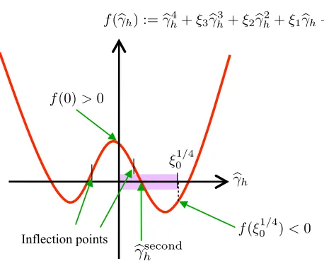
Theorem 3 Letbγsecond

h be the second largest real solution of the following quartic equation with

respect tobγh:

f(bγh):=bγ4h+ξ3bγ3h+ξ2bγ2h+ξ1bγh+ξ0=0, (23) where the coefficients are defined by

ξ3=

(L₋M)2_γ

h

LM ,

ξ2=− ξ3γh+

(L2_+M2_)η2

h

LM +

2σ4 c2

ahc 2

bh

!

,

ξ1=ξ3

p ξ0,

ξ0= η2h− σ4 c2

ahc 2

bh

!2 ,

η2_h=

1₋σ 2_L

γ2

h

1₋σ 2_M

γ2

h

γ2_h.

Then, the global VB solution can be expressed as

b

UVB≡ hBA⊤irVB_(A,B)=BbAb⊤= H

∑

h=1

bγVB

h ωbhωa⊤h,

where

bγVB

h =

( bγsecond

h ifγh>eγh,

The coefficients of the quartic equation (23) are analytic, so_bγsecond

h can also be obtained

analyt-ically, for example, byFerrari’s method (Hazewinkel, 2002).2 Therefore, the global VB solution can be analytically computed.3 This is a strong advantage over the standard ICM algorithm since many iterations and restarts would be necessary to find a good solution by ICM.

Based on the above result, the complete VB posterior can be obtained analytically as follows (the proof is also given in Appendix B):

Theorem 4 The VB posterior is given by

rVB(A,B) =

H

∏

h=1

N

M(ah;abh,σ2ahIM)

H

∏

h=1

N

L(bh;bbh,σ2bhIL), where, forbγVB

h being the solution given by Theorem 3,

b

ah=± q

bγVB

h bδh·ωah,

b

bh=± q

bγVB

h bδ−

1

h ·ωbh,

σ2_ah =− b

η2

h−σ2(M−L)

+q(ηb2

h−σ2(M−L))2+4Mσ2bη2h

2M(bγVB

h bδ−

1

h +σ2c−

2

ah )

,

σ2

bh =

− bη2

h+σ2(M−L)

+q(ηb2

h+σ2(M−L))2+4Lσ2ηb2h

2L(bγVB

h bδh+σ2c−

2

bh )

,

b δh=

(M₋L)(γh−bγVBh ) + r

(M₋L)2_(γ

h−bγVBh )2+4σ 4_LM c2

ahc2bh

2σ2_Mc−2

ah

,

b η2_h=

  

η2

h ifγh>eγh, σ4

c2

ahc2bh

otherwise.

3.3 Global Analytic Solution for Empirical VBMF

Solving the following problem gives the empirical VBMF solution:

Given σ2_∈R

++,

min FVB(A,b B,bΣA,ΣB,{c2ah,c 2

bh;h=1, . . . ,H}),

s.t. Ab_∈RM×H_,Bb_∈RL×H_,ΣA∈SH_++,ΣB∈SH_++,

(c2_ah,c2_bh)_∈R2_{++(∀h=1, . . . ,H),} whereFVB(A,b B,bΣA,ΣB,{c2ah,c

2

bh;h=1, . . . ,H})is the free energy given by Equation (20). Although this is again a non-convex optimization problem, the global optimal solution can be obtained ana-lytically. As discussed in Nakajima and Sugiyama (2011), the ratiocah/cbh is arbitrary in empirical VB. Accordingly, we fix the ratio tocah/cbh =1 without loss of generality.

2. In practice, one may solve the quartic equation numerically, for example, by the ‘roots’ function in MATLABR_.

Nakajima and Sugiyama (2011) obtained a closed form solution of the optimal hyperparame-ter value_bcahcbbh for SimpleVBMF. Therefore, we can easily obtain the global analytic solution for empirical VBMF. We have the following theorem (the proof is given in Appendix C):

Theorem 5 The global empirical VB solution is given by

b

UEVB=

H

∑

h=1

bγEVB_h ωbhωa⊤h,

where

bγEVB

h =

(

˘

γVB

h ifγh>γhand∆h≤0,

0 otherwise.

Here,

γ h= (

√

L+√M)σ, (24)

˘

c2_ahc˘2_bh= 1 2LM

γ2_h−(L+M)σ2+

q γ2

h−(L+M)σ2 2

−4LMσ4

, (25)

∆h=Mlog _γh

Mσ2˘γ VB

h +1

+Llog γh Lσ2˘γ

VB

h +1

+ 1

σ2 −2γhγ˘ VB

h +LMc˘2ahc˘ 2

bh

, (26)

and˘γVB

h is the VB solution for cahcbh =c˘ahc˘bh.

By using Theorem 3 and Theorem 5, the global empirical VB solution can be computed analyt-ically. This is again a strong advantage over the standard ICM algorithm since ICM would require many iterations and restarts to find a good local minimum. The calculation procedure for the em-pirical VB solution is as follows: After obtaining_{γh}by singular value decomposition ofV, we

first check ifγh>γ_hholds for eachh, by using Equation (24). If it holds, we compute ˘γVB_h by using

Equation (25) and Theorem 3. Otherwise,bγEVB

h =0. Finally, we check if ∆h≤0 holds by using

Equation (26).

When the noise varianceσ2_{is unknown, it may be estimated by minimizing the VB free energy} with respect toσ2_{. In practice, this single-parameter minimization may be carried out numerically} based on Equation (20) and Theorem 4.

4. Matrix Factorization for Multivariate Analysis

In this section, we explicitly describe the relation between MF and multivariate analysis techniques.

4.1 Probabilistic PCA

The relation to principal component analysis (PCA) (Hotelling, 1933) is straightforward. In proba-bilistic PCA (Tipping and Bishop, 1999), the observationv_∈RL_{is assumed to be driven by a latent} vectorea_∈RH_{in the following form:}

v=B_ea+ε.

Here,B_∈RL×H _{specifies the linear relationship betweenaeandv, andε∈R}L_{is a Gaussian noise}

Figure 1: Linear neural network.

from the latent vectorsA⊤= (a_e1, . . . ,eaM), and each latent vector is subject toae∼

N

H(0,IH). Then,

the probabilistic PCA model is written as Equations (1) and (2) withCA=IH.

If we apply Bayesian inference, the intrinsic dimension H is automatically selected without predetermination (Bishop, 1999). This useful property is calledautomatic dimensionality selection (ADS). It was shown that ADS originates from themodel-induced regularizationeffect (Nakajima and Sugiyama, 2011).

4.2 Reduced Rank Regression

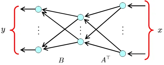
Reduced rank regression (RRR) (Baldi and Hornik, 1995; Reinsel and Velu, 1998) is aimed at learning a relation between an input vector x_∈RM _{and an output vector y∈}RL _{by using the} following linear model:

y=BA⊤x+ε, (27)

whereA_∈RM×H _andB∈RL×H_{are parameter matrices, andε∼}

_N

_L(0_,σ′2_{IL)is a Gaussian noise}

vector. This can be expressed as a linear neural network (Figure 1). Thus, we can interpret this model as first projecting the input vectorx onto a lower-dimensional latent subspace byA⊤ and then performing linear prediction byB.

Suppose we are givennpairs of input and output vectors:

V

n_={(x

i,yi)|xi∈RM,yi∈RL,i=1, . . . ,n}. (28)

Then, the likelihood of the RRR model (27) is expressed as

p(

V

n_|A,B)∝exp ₋ 1 2σ′2

n

∑

i=1

kyi−BA⊤xik2 !

. (29)

Let us assume that the samples are centered:

1 n

n

∑

i=1

xi=0 and

1 n

n

∑

i=1

yi=0.

Furthermore, let us assume that the input samples arepre-whitened(Hyv¨arinen et al., 2001), that is, they satisfy

1 n

n

∑

i=1

Let

V =ΣXY =

1 n

n

∑

i=1

yix⊤i (30)

be the samplecross-covariancematrix, and

σ2₌σ′2

n (31)

be a rescaled noise variance. Then the likelihood (29) can be written as

p(

V

n

|A,B)∝exp

−₂1_σ2kV−BA⊤k 2 Fro

exp ₋ 1 2σ2

1 n

n

∑

i=1

kyik2− kVk2Fro

!!

. (32)

The first factor in Equation (32) coincides with the likelihood of the MF model (1), and the second factor is constant with respect toAandB. Thus, RRR is reduced to MF.

However, the second factor depends on the rescaled noise varianceσ2_{, and therefore, should be} considered whenσ2_{is estimated based on the free energy minimization principle. Furthermore, the} normalization constant of the likelihood (29) is slightly different from that of the MF model. Taking into account of these differences, the VB free energy of the RRR model (29) with the priors (2) and (3) is given by

FVB−RRR=logrA(A) +logrB(B)−logp(

V

n|A,B)p(A)p(B)_r(A)r(B)

=∑

n

i=1kyik2

2nσ2 + nL

2 logσ 2₊M

2 log

|CA| |ΣA|

+L 2log

|CB| |ΣB|

+1 2tr

n

C_A−1

b

A⊤Ab+MΣA

+C−1

B

b

B⊤Bb+LΣB

+σ−2_−2Ab⊤_V⊤_Bb+Ab⊤_Ab+MΣ A

b

B⊤Bb+LΣB o

+const. (33)

Note that the difference from Equation (20) exists only in the first two terms. Minimizing Equa-tion (33), instead of EquaEqua-tion (20), gives an estimator for the rescaled noise variance. For the standard ICM algorithm, the following update rule should be substituted for Equation (14):

(σ2)RRR=

n−1∑n_i=1kyik2−tr(2V⊤BbAb⊤) +tr

(Ab⊤Ab+MΣA)(Bb⊤Bb+LΣB)

nL . (34)

Once the rescaled noise varianceσ2_{is estimated, Equation (31) gives the original noise varianceσ}′2 of the RRR model (29).

4.3 Partial Least-Squares

Partial least-squares(PLS) (Worsley et al., 1997; Rosipal and Kr¨amer, 2006) is similar to RRR. In PLS, the parametersAandBare learned so that the squared Frobenius norm of the difference from the samplecross-covariance matrix(30) is minimized:

(A,B):=argmin

A,B k

ΣXY−BA⊤k2Fro. (35)

4.4 Canonical Correlation Analysis

For paired samples (28), the goal ofcanonical correlation analysis(CCA) (Hotelling, 1936; Ander-son, 1984) is to seek vectorsa_∈RM_andb∈RL_{such that the correlation betweena}⊤_xandb⊤_yis

maximized.aandbare calledcanonical vectors.

More formally, given the first(h₋1)canonical vectorsa1, . . . ,ah−1andb1, . . . ,bh−1, theh-th canonical vectors are defined as

(ah,bh):=argmax

a_,b

a⊤ΣXYb p

a⊤ΣX Xa p

b⊤ΣYYb

,

s.t.a⊤ΣX Xah′ =0 and b⊤ΣYYbh′=0 forh′=1, . . . ,h−1,

where ΣX X andΣYY are the sample covariance matrices ofx andy, respectively, and ΣXY is the

sample cross-covariance matrix, defined in Equation (30), of x andy. The entire solution A= (a1, . . . ,aH)andB= (b1, . . . ,bH)are given as theHlargest singular vectors ofΣ−X X1/2ΣXYΣYY−1/2.

Let us assume that xandy are both pre-whitened, that is,ΣX X =IM andΣYY =IL. Then the

solutionsA andBare given as the singular vectors ofΣXY associated with theH largest singular

values. Since the solutions of Equation (35) are also given by theH dominant singular vectors of

ΣXY (Stewart, 1993), CCA is reduced to the maximum likelihood estimation of the MF model (1).

5. Experimental Results

In this section, we show experimental results on artificial and benchmark data sets, which illustrate practical usefulness of our analytic solution.

5.1 Experiment on Artificial Data

We compare the standard ICM algorithm and theanalyticsolution in the empiricalVB scenario with unknown noise variance, that is, the hyperparameters(CA,CB) and the noise varianceσ2 are

also estimated from observation. We use the full-rank model (i.e.,H=min(L,M)), and expect the ADS effect to automatically find the true rankH∗.

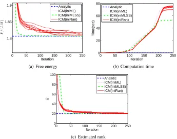
Figure 2 shows the free energy, the computation time, and the estimated rank over iterations for an artificial (Artificial1) data set with the data matrix sizeL=100 andM=300, and the true rank H∗=20. We randomly createdtruematricesA∗_∈RM×H∗ _andB∗_∈RL×H∗ _{so that each entry ofA}∗ andB∗ follows

N

1(0,1). An observed matrixV was created by adding a noise subject to

N

1(0,1) to each entry ofB∗A∗⊤.

The standard ICM algorithm consists of the update rules (8)–(14). Initial values were set in the following way: AbandBbare randomly created so that each entry follows

N

1(0,1). Other variables are set toΣA=ΣB=CA=CB=IH andσ2=1. Note that we rescaleV so thatkVk2Fro/(LM) =1, before starting iterations. We ran the standard ICM algorithm 10 times, starting from different initial points, and each trial is plotted by a solid line (labeled as ‘ICM(iniRan)’) in Figure 2. The analytic solution consists of applying Theorem 5 combined with a naive 1-dimensional search for the estimation of noise varianceσ2_{. The analytic solution is plotted by the dashed line (labeled as} ‘Analytic’). We see that the analytic solution estimates the true rankHb =H∗=20 immediately (_∼0.1 sec on average over 10 trials), while the ICM algorithm does not converge in 60 sec.

0 50 100 150 200 250 1.8

1.85 1.9

Iteration

F

/

(

L

M

)

Analytic ICM(iniML) ICM(iniMLSS) ICM(iniRan)

(a) Free energy

0 50 100 150 200 250

0 20 40 60 80

Iteration

Time(sec)

Analytic ICM(iniML) ICM(iniMLSS) ICM(iniRan)

(b) Computation time

0 50 100 150 200 250

0 20 40 60 80 100

Iteration

bH

Analytic ICM(iniML) ICM(iniMLSS) ICM(iniRan)

(c) Estimated rank

Figure 2: Experimental results for Artificial1data set, where the data matrix size is L=100 and M=300, and the true rank isH∗=20.

minima. We empirically observed that the local minima problem tends to be more critical, whenH∗ is large (close toH).

We also evaluated the ICM algorithm with different initialization schemes. The line labeled as ‘ICM(iniML)’ indicates the ICM algorithm starting from the maximum likelihood (ML) solution: (a_bh,bbh) = (√γ_hωah,

√_γ

hωbh). The initial values for other variables are the same as the random initialization. Figures 2 and 3 show that the ML initialization generally makes convergence faster than the random initialization, but suffers from the local minima problem more often.

We observed that starting from a small noise variance tends to alleviate the local minima prob-lem at the expense of slightly slower convergence. The line labeled as ‘ICM(iniMLSS)’ indicates the ICM algorithm starting from the ML solution with a small noise varianceσ2_{=0.0001. We see} in Figures 2 and 3 that this initialization improves quality of solutions, and successfully finds the true rank for these artificial data sets. However, we will show in Section 5.2 that this scheme still suffers from the local minima problem on benchmark data sets.

5.2 Experiment on Benchmark Data

0 50 100 150 200 250 2.4

2.5 2.6 2.7 2.8 2.9 3

Iteration

F

/

(

L

M

)

Analytic ICM(iniML) ICM(iniMLSS) ICM(iniRan)

(a) Free energy

0 50 100 150 200 250

0 10 20 30 40

Iteration

Time(sec)

Analytic ICM(iniML) ICM(iniMLSS) ICM(iniRan)

(b) Computation time

0 50 100 150 200 250

0 20 40 60 80

Iteration

bH

Analytic ICM(iniML) ICM(iniMLSS) ICM(iniRan)

(c) Estimated rank

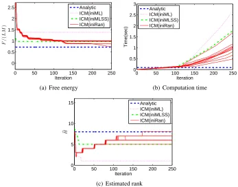
Figure 3: Experimental results forArtificial2data set (L=70,M=300, andH∗=40).

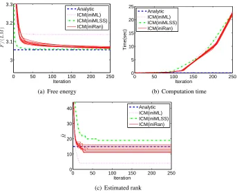
at local minima with wrong ranks;4 ‘ICM(iniML)’ converges slightly faster but to worse local minima; ‘ICM(iniMLSS)’ tends to give better solutions. Unlike in the artificial data experiment, ‘ICM(iniMLSS)’ fails to find thecorrectrank with these benchmark data sets. We also conducted experiments on other benchmark data sets, and found that the ICM algorithm generally converges slowly, and sometimes suffers from the local minima problem, while our analytic-form gives the global solution immediately.

Finally, we applied VBMF to areduced rank regression(RRR) (Reinsel and Velu, 1998) task, and show the results in Figure 7. We centered the L=3-dimensional outputs and the M= 7-dimensional inputs of the Concrete Slump Test data set, and pre-whitened the inputs. We also standardized the outputs so that the variance of each element is equal to one. Note that we have to minimize Equation (33), instead of Equation (20), for estimating the noise variance in our proposed method with the analytic solution, and use Equation (34), instead of Equation (14), for updating the noise variance in the standard ICM algorithm.

Overall, the proposed global analytic solution is shown to be a useful alternative to the standard ICM algorithm.

0 50 100 150 200 250 0

0.5 1 1.5 2 2.5

Iteration

F

/

(

L

M

)

Analytic ICM(iniML) ICM(iniMLSS) ICM(iniRan)

(a) Free energy

0 50 100 150 200 250

0 0.5 1 1.5 2 2.5 3

Iteration

Time(sec)

Analytic ICM(iniML) ICM(iniMLSS) ICM(iniRan)

(b) Computation time

0 50 100 150 200 250

0 5 10 15

Iteration

bH

Analytic ICM(iniML) ICM(iniMLSS) ICM(iniRan)

(c) Estimated rank

Figure 4: PCA results for theGlassdata set (L=9,M=214).

6. Discussion

In this section, we first derive simple analytic-form solutions for special cases, where the model-induced regularization and the prior-induced regularization can be clearly distinguished (Section 6.1). Then, we discuss the relation between model pruning by VB and spontaneous sym-metry breaking (Section 6.2). Finally, we consider possibilities of extending our results to more general cases (Section 6.3).

6.1 Special Cases

Here, we consider two special cases, where simple-form solutions are obtained.

6.1.1 FLATPRIOR

Whencahcbh→∞(i.e., the prior isalmostflat), a simple-form exact solution for SimpleVBMF has been obtained in Nakajima and Sugiyama (2011). Thanks to Theorem 1, the same applies to VBMF under the standardmatrix-wise independence assumption. This solution can be obtained also by factorizing the quartic equation (23) as follows:

lim

c_ahc_bh→∞f(bγh) =

bγh+

M L

1₋σ 2_L

γ2

h

γh

bγh+

1₋σ 2_M

γ2

h

γh

·

bγh−

1₋σ 2_M

γ2

h

γh

bγh−

M L

1₋σ 2_L

γ2

h

γh

0 50 100 150 200 250 2.4

2.5 2.6 2.7 2.8 2.9 3

Iteration

F

/

(

L

M

)

Analytic ICM(iniML) ICM(iniMLSS) ICM(iniRan)

(a) Free energy

0 50 100 150 200 250

0 2000 4000 6000 8000

Iteration

Time(sec)

Analytic ICM(iniML) ICM(iniMLSS) ICM(iniRan)

(b) Computation time

0 50 100 150 200 250

0 10 20 30 40 50

Iteration

bH

Analytic ICM(iniML) ICM(iniMLSS) ICM(iniRan)

(c) Estimated rank

Figure 5: PCA results for theSatimagedata set (L=36,M=6435).

0 50 100 150 200 250

3 3.1 3.2 3.3

Iteration

F

/

(

L

M

)

Analytic ICM(iniML) ICM(iniMLSS) ICM(iniRan)

(a) Free energy

0 50 100 150 200 250

0 5 10 15 20 25

Iteration

Time(sec)

Analytic ICM(iniML) ICM(iniMLSS) ICM(iniRan)

(b) Computation time

0 50 100 150 200 250

0 10 20 30 40

Iteration

bH

Analytic ICM(iniML) ICM(iniMLSS) ICM(iniRan)

(c) Estimated rank

0 50 100 150 200 250 −2.0435

−2.0434 −2.0433 −2.0432 −2.0431 −2.043

Iteration

F

/

(

n

L

)

Analytic ICM(iniML) ICM(iniMLSS) ICM(iniRan)

(a) Free energy

0 50 100 150 200 250

0 0.02 0.04 0.06 0.08

Iteration

Time(sec)

Analytic ICM(iniML) ICM(iniMLSS) ICM(iniRan)

(b) Computation time

0 50 100 150 200 250

0 1 2 3 4

Iteration

bH

Analytic ICM(iniML) ICM(iniMLSS) ICM(iniRan)

(c) Estimated rank

Figure 7: RRR results for theConcrete Slump Testdata set (L=3,M=7).

Since Theorem 3 states that its second largest solution gives the VB estimator for

γh>limc_ahc_bh→∞eγh= √

Mσ2_{, we have the following corollary:}

Corollary 1 The global VB solution with the almost flat prior (i.e., cahcbh →∞) is given by

lim

c_ahc_bh→∞bγ

VB

h =bγPJSh =     

max

0,

1₋Mσ 2

γ2

h

γh

ifγh>0,

0 otherwise.

(36)

Equation (36) is the positive-part James-Stein (PJS) shrinkage estimator (James and Stein, 1961), operated on each singular component separately. This is actually the upper-bound of the VB solution for arbitrarycahcbh >0. The counter-intuitive fact—a shrinkage is observed even in the limit of flat priors—can be explained by strong non-uniformity of thevolume element of the Fisher metric, that is, theJeffreysprior (Jeffreys, 1946), in the parameter space. This effect is called model-induced regularization(MIR), because it is induced not by priors but by the structure of the model likelihood function (Nakajima and Sugiyama, 2011). MIR was shown to generally appear in Bayesian estimation when the model isnon-identifiable(i.e., the mapping between parameters and distribution functions is not one-to-one) (Watanabe, 2009). The mechanism how non-identifiability causes MIR and ADS in VBMF was explicitly illustrated in Nakajima and Sugiyama (2011).

6.1.2 SQUAREMATRIX

equation with respect to_bγ2

h (Nakajima and Sugiyama, 2011). We can also find the solution by

factorizing the quartic equation (23) forγh> √

Mσ2_{as follows:} fsquare(bγh) =

bγh+bγPJSh + σ2 cahcbh

bγh+bγPJSh − σ2 cahcbh

·

bγh−bγPJSh + σ2 cahcbh

bγh−bγPJSh − σ2 cahcbh

=0.

Using Theorem 3, we have the following corollary:

Corollary 2 When L=M, the global VB solution is given by

bγVB_h −square=max

0,bγPJS_{h −} σ

2 cahcbh

. (37)

Equation (37) shows that, in this case, MIR andprior-induced regularization(PIR) can be com-pletely decomposed—the estimator is equipped with themodel-induced PJS shrinkage (bγPJS

h ) and

theprior-inducedtrace-norm shrinkage (₋σ2_/(c

ahcbh)).

The empirical VB solution is also simplified in this case. The following corollary is obtained simply by combining Theorem 1 in this paper and Corollary 2 in Nakajima and Sugiyama (2011):

Corollary 3 When L=M, the global empirical VB solution is given by

bγEVB_h =

    

1₋Mσ 2

γ2

h −ρ₋

γh ifγh>γ_hand∆′_h≤0,

0 otherwise,

where

γ h=2

√

Mσ,

∆′_h=log

_γ2

h

Mσ2(1−ρ−)

− γ

2

h

Mσ2(1−ρ−) +

1+ γ 2

h

2Mσ2ρ 2

+

,

ρ_±=

v u u t1

2 1− 2Mσ2

γ2

h ±

s

1₋4Mσ 2

γ2

h !

.

By using Corollary 2 and Corollary 3, respectively, we can easily compute the VB and the empirical VB solutions in this case without a quartic solver.

6.2 Model Pruning and Spontaneous Symmetry Breaking

0.1 0.1 0.1 0.1 0.1 0.1 0.1 0.1 0.2 0.2 0.2 0.2 0.2 0.2 0.2 0.2 0.3 0.3 0.3 0.3 0.3 0.3 0.3 0.3 A B

Bayes p osterior (V = 0)

−3 −2 −1 0 1 2 3

−3 −2 −1 0 1 2 3 MAP estimator: (A, B) = (0,0)

0.1 0.1 0.1 0.1 0.1 0.1 0.1 0.1 0.2 0.2 0.2 0.2 0.2 0.2 0.2 0.2 0.2 0.2 0.3 0.3 0.3 0.3 0.3 0.3 0.3 0.3 0.3 0.3 A B

Bayes p osterior (V= 1)

−3 −2 −1 0 1 2 3

−3 −2 −1 0 1 2 3 MAP estimators: (A, B)≈ (±1,_±1)

0.1 0.1 0.1 0.1 0.1 0.1 0.1 0.1 0.2 0.2 0.2 0.2 0.2 0.2 0.2 0.2 0.3 0.3 0.3 0.3 0.3 0.3 0.3 0.3 A B

Bayes p osterior (V = 2)

−3 −2 −1 0 1 2 3

−3 −2 −1 0 1 2 3 MAP estimators: (A, B)≈(±√2,_±√2)

0.05 0.05 0.05 0.05 0.05 0.05 0.05 0.1 0.1 0.1 0.1 0.15 0.15 A B

VB p osterior (V = 0)

−3 −2 −1 0 1 2 3

−3 −2 −1 0 1 2 3

VB estimator : (A, B) = (0,0)

0.05 0.05 0.05 0.05 0.05 0.05 0.05 0.1 0.1 0.1 0.1 0.15 0.15 A B

VB p osterior (V= 1)

−3 −2 −1 0 1 2 3

−3 −2 −1 0 1 2 3

VB estimator : (A, B) = (0,0)

0.05 0.05 0.05 0.05 0.05 0.05 0.1 0.1 0.1 0.1 0.1 0.15 0.15 0.15 0.15 0.2 0.2 0.2 0.25 0.25 0.3 A B

VB p osterior (V = 2)

−3 −2 −1 0 1 2 3

−3 −2 −1 0 1 2 3

VB estimator : (A, B)≈ (√1.5,√1.5)

Figure 8: Bayes posteriors (top row) and the VB posteriors (bottom row) of ascalar factorization model (i.e., a MF model forL=M=H=1) with σ2_{=1 and c}

a=cb=100 (almost

flat priors), when the observed values areV =0 (left),V =1 (middle), andV =2 (right), respectively. In the top row, the asterisks indicate the MAP estimators, and the dashed lines the ML estimators (the modes of the contour). In the bottom row, the asterisks indicate the VB estimators. All graphs are quoted from Nakajima and Sugiyama (2011).

In VBMF, degrees of freedom are pruned when spontaneous symmetry breaking doesnotoccur. Figure 8 shows the Bayes posteriors (top row) and the VB posteriors (bottom row) of a scalar factorizationmodel (i.e., a MF model forL=M=H=1) withσ2_{=1 andc}

a=cb=100 (almost

flat priors). As we can see in the top row, the Bayes posterior has two modes unlessV =0, and the distance between the two modes increases as _|V_| increases. Since the VB posterior tries to approximate the Bayes posterior with a single uncorrelated distribution, it stays at the origin when

|V_|is not sufficiently large. When _|V_|is large enough, the VB posterior approximates one of the modes, as seen in the graphs in the right column (for the case whenV =2) of Figure 8 (note that there also exists anequivalentVB solution located at(A,B)_≈(₋√1.5,₋√1.5)).

Equation (36) implies that symmetry breaking occurs whenV >eγh∼ √

a different transition point, and tends to give a sparser solution (see Section 4 in Nakajima and Sugiyama (2011) for further discussion).

Given that the rigorous Bayesian estimator in MF is not sparse (see Figure 10 in Nakajima and Sugiyama, 2011), one might argue that the sparsity of VBMF is inappropriate. On the other hand, given that model pruning by VB has been acknowledged as a practically useful property, one might also argue thatappropriatenessshould be measured in terms of performance. Motivated by the latter idea, we have conducted performance analysis of EVBMF in our latest work (Nakajima et al., 2012b), and shown that model pruning by EVBMF works perfectly under some condition. Conducting performance analysis in other models would be our future work.

6.3 Extensions

In this paper, we derived the global analytic solution of VBMF, by fully making use of the assump-tions that the likelihood and priors are both spherical Gaussian, and that the observed matrix has no missing entry. They were necessary to solve the free energy minimization problem as a reweighted SVD. In this subsection, we discuss possibilities to extend our results to more general problems.

6.3.1 ROBUSTPCA

VBMF gives a low-rank solution, which can be seen as a singular-component-wise sparse solution. We can extend our analysis so that a wider variety of sparsity can be handled.

Robust PCA (Candes et al., 2009) has recently gathered a great deal of attention. Equipped with an element-wise sparse term in addition to a low-rank term, robust PCA separates the low dimensional data structure from spiky noise. Its VB variant has also been proposed (Babacan et al., 2012). To obtain the VB solution of robust PCA, we have proposed a novel algorithm where the analytic VBMF solution is applied to partial problems (Nakajima et al., 2012a). Although the global optimality is not guaranteed, this algorithm has been experimentally shown to give a better solution than the standard ICM algorithm. In addition, our proposed algorithm can handle a variety of sparse terms beyond robust PCA.

6.3.2 TENSORFACTORIZATION

We have shown that the VB solution undermatrix-wise independence essentially agrees with the SimpleVB solution under column-wise independence. We expect that similarredundancywould be found also in other models, for example,tensor factorization(Kolda and Bader, 2009; Carroll and Chang, 1970; Harshman, 1970; Tucker, 1996). In our preliminary study so far, we saw that the analytic VB solution for tensor factorization is not attainable, at least in the same way as MF. However, we have found that the optimal solution has diagonal covariances for the core tensor in Tucker decomposition (Nakajima, 2012), which would allow us to greatly simplify inference algorithms and reduce necessary memory storage and computational costs.

6.3.3 CORRELATEDPRIORS

the free energy (20) is invariant under the following transformation for anyT:

A_→AT⊤, ΣA→TΣAT⊤, CA→TCAT⊤,

B_→BT−1, ΣB→(T−1)TΣBT−1, CB→(T−1)⊤CBT−1.

Accordingly, the following procedure gives the global solution analytically: the analytic solution given the diagonal(C_A′,C_B′)is first computed, and the above transformation is then applied.

Handling priors correlated over rows of A and B is more challenging and remains as future work. Such a prior allows model correlations in the observation space, and can capture useful characteristics of data, for example, short-term correlation in time-series data and correlation among neighboring pixels in image data.

6.3.4 MISSINGENTRIESPREDICTION

Missing entries prediction is another prototypical application of MF (Konstan et al., 1997; Funk, 2006; Lim and Teh, 2007; Ilin and Raiko, 2010; Salakhutdinov and Mnih, 2008), where finding the global VBMF solution seems a very hard problem. However, one may use our analytic solution as a subroutine, for example, in thesoft-thresholdingstep of SOFT-IMPUTE(Mazumder et al., 2010). Along this line, Seeger and Bouchard (2012) have recently proposed an algorithm, which tends to give a better local solution than the standard ICM algorithm for missing entries prediction. They also proposed a way to cope with non-Gaussian likelihood functions.

7. Conclusion

Overcoming the non-convexity of VB methods has been one of the important challenges in the Bayesian machine learning community, since it sometimes prevented us from applying the VB methods to highly complex real-world problems. In this paper, we focused on the matrix factor-ization (MF) problem with no missing entry, and showed that this weakness could be overcome by analyticallycomputing the global optimal solution. We further derived the global optimal solution analytically for the empirical VBMF method, where hyperparameters are also optimized based on data samples. Since no hand-tuning parameter remains in empirical VBMF, our analytic-form solu-tion is practically useful and computasolu-tionally highly efficient. Numerical experiments showed that the proposed approach is promising.

We discussed the possibility that our analytic solution can be used as a building block of novel algorithms for more general problems. Tackling such possible extensions and conducting perfor-mance analysis of those methods are our future work.

Acknowledgments

Appendix A. Proof of Theorem 1

In the same way as in the analysis for the SimpleVB approximation (see the proof of Lemma 10 in Nakajima and Sugiyama, 2011), we can show that any minimizer of the free energy (20) is a stationary point. Therefore, Equations (8)–(11) hold for any solution.

We consider the following three cases:

Case 1 When no pair of diagonal entries ofCACBcoincide.

Case 2 When all diagonal entries ofCACBcoincide.

Case 3 When (not all but) some pairs of diagonal entries ofCACBcoincide.

In the following, we prove that, in Case 1,ΣAandΣBare diagonal for any solution(A,bB,b ΣA,ΣB),

and that, in other cases, any solution has itsequivalentsolution with diagonalΣAandΣB.

Our proof relies on a technique related to the following proposition:

Proposition 6 (Ruhe, 1970) Let λh(Φ),λh(Ψ) be the h-th largest eigenvalues of positive-definite

symmetric matricesΦ,Ψ_∈RH×H_{, respectively. Then, it holds that}

tr_{Φ−1_Ψ

} ≥ H

∑

h=1

λh(Ψ) λh(Φ)

.

We use the following lemma (its proof is given in Appendix D.1):

Lemma 7 LetΓ,Ω,Φ_∈RH×H_{be a non-degenerate diagonal matrix, an orthogonal matrix, and a} symmetric matrix, respectively. Let_{Λ(k)_,Λ′(k)_∈RH×H_{;k=1, . . . ,K}be arbitrary diagonal}

matri-ces. If

G(Ω) =tr

(

ΓΩΦΩ⊤+

K

∑

k=1

Λ(k)_ΩΛ′(k)_Ω⊤ )

(38)

is minimized (as a function ofΩ, givenΓ,Φ,_{Λ(k)_,Λ′(k)_{}) whenΩ=I}

H, thenΦis diagonal. Here,

K can be any natural number including K=0(when only the first term exists).

A.1 Proof for Case 1

Here, we consider the case when cahcbh >cah′cbh′ for any pair h<h′. We will show that any minimizer has diagonal covariances in this case.

Assume that(A∗_,B∗_,Σ∗

A,Σ∗B)is a minimizer of the free energy (20), and consider the following

variation from it with respect to an arbitraryH_×Horthogonal matrixΩ:

b

A=A∗C_A−1/2Ω⊤C_A1/2, (39)

b

B=B∗C_A1/2Ω⊤C−_A1/2, (40)

ΣA=CA1/2ΩC−

1/2

A Σ∗AC−

1/2

A Ω⊤C

1/2

A , (41)

ΣB=C_A−1/2ΩC_A1/2Σ∗BC

1/2

A Ω⊤C−

1/2

Note that this variation does not change BbAb⊤, and that (A,b B,bΣA,ΣB) = (A∗,B∗,Σ∗A,Σ∗B) holds if Ω=IH. Then, the free energy (20) can be written as a function ofΩ:

FVB(Ω) =1 2tr

n

C_A−1C_B−1ΩC_A1/2B∗⊤B∗+LΣ∗_BC_A1/2Ω⊤o+const. (43) (the terms except the second term in the curly braces in Equation (20) are constant).

We define

Φ=C_A1/2B∗⊤B∗+LΣ∗_BC1_A/2, and rewrite Equation (43) as

FVB(Ω) =1 2tr

n

C_A−1C−_B1ΩΦΩ⊤o+const. (44) The assumption that (A∗_,B∗_,Σ∗

A,Σ∗B) is a minimizer requires that Equation (44) is minimized

whenΩ=IH. Then, Lemma 7 (forK=0) implies thatΦis diagonal.5 Therefore,

C−_A1/2ΦC_A−1/2(=ΦC_A−1) =B∗⊤B∗+LΣ∗_B

is also diagonal. Consequently, Equation (10) implies thatΣ∗

Ais diagonal.

Next, consider the following variation with respect to an arbitraryH_×H orthogonal matrixΩ′,

b

A=A∗C_B1/2Ω′⊤C_B−1/2,

b

B=B∗C_B−1/2Ω′⊤C1_B/2,

ΣA=C−_B1/2Ω′C1_B/2Σ∗AC

1/2

B Ω′⊤C −1/2

B ,

ΣB=C1B/2Ω′C−

1/2

B Σ∗BC−

1/2

B Ω′⊤C

1/2

B .

Then, the free energy as a function ofΩ′_{is given by}

FVB(Ω′) =1 2tr

n

C_A−1C−_B1Ω′C1_B/2A∗⊤A∗+MΣ∗_AC_B1/2Ω′⊤o+const.

From this, we can similarly prove thatΣ∗_Bis also diagonal, which completes the proof for Case 1.

A.2 Proof for Case 2

Here, we consider the case whenCACB =cIH for some positive c∈R. In this case, there exist

solutions with non-diagonal covariances. However, any of them belongs to an equivalent class involving a solution with diagonal covariances.

We can easily show that the free energy (20) is invariant ofΩunder the transformation (39)– (42). This arbitrariness forms anequivalentclass of solutions. Since there existsΩthat diagonalizes any givenΣ∗_Athrough Equation (41), eachequivalentclass involves a solution with diagonalΣA. In

the following, we will prove that any solution with diagonalΣAhas diagonalΣB.

Assume that(A∗_,B∗_,Σ∗

A,Σ∗B)is a solution with diagonalΣ∗A, and consider the following variation

from it with respect to an arbitraryH_×Horthogonal matrixΩ:

b

A=A∗C−_A1/2Γ−1/2Ω⊤Γ1/2C_A1/2,

b

B=B∗C1_A/2Γ1/2_Ω⊤_Γ−1/2_C−1/2

A ,

ΣA=CA1/2Γ1/2ΩΓ−1/2C−

1/2

A Σ∗AC−

1/2

A Γ−1/2Ω⊤Γ1/2C

1/2

A , ΣB=C−

1/2

A Γ−

1/2_ΩΓ1/2_C1/2

A Σ∗BC

1/2

A Γ

1/2_Ω⊤Γ−1/2_C−1/2

A .

Here,Γ=diag(γ1, . . . ,γH)is an arbitrary non-degenerate (γh6=γh′ forh6=h′) positive-definite

diag-onal matrix. Then, the free energy can be written as a function ofΩ:

FVB(Ω) = 1 2tr

n

ΓΩΓ−1/2C_A−1/2A∗⊤A∗+MΣ_A∗C_A−1/2Γ−1/2Ω⊤

+c−1Γ−1ΩΓ1/2C_A1/2B∗⊤B∗+LΣ∗_BC_A1/2Γ1/2Ω⊤o. (45) We define

ΦA=Γ−1/2C−_A1/2

A∗⊤A∗+MΣ∗_AC_A−1/2Γ−1/2,

ΦB=c−1Γ1/2C1A/2

B∗⊤B∗+LΣ∗_BC_A1/2Γ1/2_, and rewrite Equation (45) as

FVB(Ω) =1 2tr

n

ΓΩΦAΩ⊤+Γ−1ΩΦBΩ⊤ o

. (46)

Since Σ∗

A is diagonal, Equation (10) implies that ΦB is diagonal. The assumption that

(A∗,B∗,Σ∗_A,Σ∗_B)is a solution requires that Equation (46) is minimized when Ω=IH. Accordingly,

Lemma 7 implies thatΦAis diagonal. Consequently, Equation (11) implies thatΣ∗Bis diagonal.

Thus, we have proved that any solution has itsequivalent solution with diagonal covariances, which completes the proof for Case 2.

A.3 Proof for Case 3

Finally, we consider the case whencahcbh =ca′_hcbh′ for (not all but) some pairs h6=h

′_{. First, in}

the same way as for Case 1, we can prove that ΣA andΣB are block diagonal where the blocks

correspond to the groups sharing the samecahcbh. Next, we can apply the proof for Case 2 to each block, and show that any solution has itsequivalentsolution with diagonalΣAandΣB. Combining

these results completes the proof of Theorem 1.

A.4 General Expression

In summary, for any minimizer of Equation (20), the covariances can be written in the following form:

ΣA=CA1/2ΘC−

1/2

A ΓΣAC

−1/2

A Θ⊤C

1/2

A (=C−

1/2

B ΘC

1/2

B ΓΣAC 1/2

B Θ⊤C−

1/2

B ), (47)

ΣB=C_A−1/2ΘC_A1/2ΓΣBC 1/2

A Θ⊤C−

1/2

A (=C

1/2

B ΘC−

1/2

B ΓΣBC

−1/2

B Θ⊤C

1/2