On Semi-Supervised Linear Regression in
Covariate Shift Problems
Kenneth Joseph Ryan [email protected]
Mark Vere Culp [email protected]
Department of Statistics West Virginia University Morgantown, WV 26506, USA
Editor:Xiaotong Shen
Abstract
Semi-supervised learning approaches are trained using the full training (labeled) data and available testing (unlabeled) data. Demonstrations of the value of training with unlabeled data typically depend on a smoothness assumption relating the conditional expectation to high density regions of the marginal distribution and an inherent missing completely at random assumption for the labeling. So-called covariate shift poses a challenge for many existing semi-supervised or supervised learning techniques. Covariate shift models allow the marginal distributions of the labeled and unlabeled feature data to differ, but the conditional distribution of the response given the feature data is the same. An example of this occurs when a complete labeled data sample and then an unlabeled sample are obtained sequentially, as it would likely follow that the distributions of the feature data are quite different between samples. The value of using unlabeled data during training for the elastic net is justified geometrically in such practical covariate shift problems. The approach works by obtaining adjusted coefficients for unlabeled prediction which recalibrate the supervised elastic net to compromise: (i) maintaining elastic net predictions on the labeled data with (ii) shrinking unlabeled predictions to zero. Our approach is shown to dominate linear supervised alternatives on unlabeled response predictions when the unlabeled feature data are concentrated on a low dimensional manifold away from the labeled data and the true coefficient vector emphasizes directions away from this manifold. Large variance of the supervised predictions on the unlabeled set is reduced more than the increase in squared bias when the unlabeled responses are expected to be small, so an improved compromise within the bias-variance tradeoff is the rationale for this performance improvement. Performance is validated on simulated and real data.
Keywords: joint optimization, semi-supervised regression, usefulness of unlabeled data
1. Introduction
L L L L
L L
L L
L L L L L L
L L L L
L L
L L
L L
L L
L L
L L
L U
U U U UU
U U U
U
U
U U
U
U U
U U
U U
U U U
U U
U
U U
U U
U U
U U U
U
U U
U U
U U U
U U
U U U
U U U
U U U
U U U
U UU
UU U U
U U
U U U
x1 x2
Labeled Data
Unlabeled Data
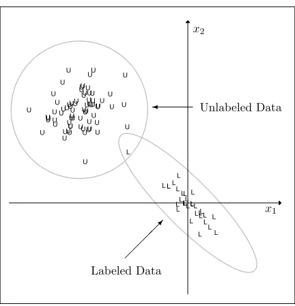
Figure 1: These feature data withp= 2 are referred to as the “block extrapolation” example because the unlabeled data “block” the 1st principal component of the labeled data. It is informative to think about how ridge regression would predict the unlabeled cases in this example. Favoring shrinking along the 2nd component will lead to high prediction variability. These block data are the primary working example throughout Sections 2-5, and it will be demonstrated that our semi-supervised approach has a clear advantage.
2005; Aswani et al., 2010). Many techniques including manifold regularization (Belkin et al., 2006) and graph cutting approaches (Wang et al., 2013) were developed to capitalize on unlabeled information during training, but beneath the surface of nearly all this work is the implicit or explicit use of MCAR (Lafferty and Wasserman, 2007).
Covariate shift is a different paradigm for semi-supervised learning (Moreno-Torres et al., 2008). It stipulates that the conditional distribution of the label given the feature data does not depend on the missingness of a label, but that the feature data distribution may depend on the missingness of a label. As a consequence, feature distributions can differ between labeled and unlabeled sets. Attempting to characterize smoothness assumptions between the regression function and the marginal of X (Azizyan et al., 2013) may not realize the value of unlabeled data if an implicit MCAR assumption breaks down. Instead, its value is in shrinking regression coefficients in an ideal direction to optimize the bias-variance tradeoff on unlabeled predictions. This is a novelty of our research direction.
to permeate the drug (Mente and Lombardo, 2005). Attributes can take years to obtain, while the feature information can be obtained much faster. As a result, the labeled data are often measurements on drugs with known attributes while the unlabeled data are usually compounds with unknown attributes that may potentially become new drugs (marketed to the public). Other applications mostly in classification include covariate shift problems (Yamazaki et al., 2007), reject inference problems from credit scoring (Moreno-Torres et al., 2008), spam filtering and brain computer interfacing (Sugiyama et al., 2007), and gene expression profiling of microarray data (Gretton et al., 2009). Gretton et al. (2009) further note that covariate shift occurs often in practice, but is under reported in the machine learning literature.
Many of the hypothetical examples to come do not conform to MCAR. The Figure 1 fea-ture data are used to illustrate key concepts as they are developed in this work. Its labeled and unlabeled partitioning is unlikely if responses are MCAR. The vector of supervised ridge regression coefficients is proportionally shrunk more along the lower order principal component directions (Hastie et al., 2009). Such shrinking is toward a multiple of the unla-beled data centroid in the hypothetical Figure 1 scenario, so ridge regression may not deflate the variance of the unlabeled predictions enough. Standard methods for tuning parameter estimation via cross-validation do not account for the distribution of the unlabeled data either. Thus, supervised ridge regression is at a distinct disadvantage by not accounting for the unlabeled data during optimization. In general, the practical shortcoming of supervised regression (e.g., ridge, lasso, or elastic net) is to define regression coefficients that predict well for any unlabeled configuration. Our main contribution to come is a mathematical framework for adapting a supervised estimate to the unlabeled data configuration at hand for improved performance. It also provides interpretable “extrapolation” adjustments to the directions of shrinking as a byproduct.
Culp (2013) proposed a joint trained elastic net for semi-supervised regression under MCAR. The main idea was to use the joint training problem that encompasses the S3VM (Chapelle et al., 2006a) and ψ-learning (Wang et al., 2009) to perform semi-supervised elastic net regression. The concept was that the unlabeled data should help with decorrela-tion and variable selecdecorrela-tion, two known hallmarks of the supervised elastic net extended to semi-supervised learning (Zou and Hastie, 2005). Culp (2013), however, did not contain a complete explanation of how exactly the approach used unlabeled data and under what set of mathematical assumptions it is expected to be useful.
The joint trained elastic net framework is strengthened in this paper to handle covariate shift. Rigorous geometrical and theoretical arguments are given for when it is expected to work. Circumstances where the feature data distribution changes by label status is the primary setting. One could view the unlabeled data as providing a group of extrapola-tions (or a separate manifold) from the labeled data. Even if responses are MCAR, the curse of dimensionality stipulates that nearly all predictions from a supervised learner are extrapolations in higher dimensions (Hastie et al., 2009), so the utility of the proposed semi-supervised approach is likely to increase with p.
Presentation of major concepts often begins with hypothetical, graphical examples in
shift before diving into the more rigorous mathematics in later sections. The problem is set-up formally in Section 3. The nature of regularization approaches (e.g., ridge, lasso, and elastic net) is studied with emphasis on a geometric perspective in Section 4. The geometry helps articulate realistic assumptions for the theoretical risk results in Section 5, and the theoretical risk results help define informative simulations and real data tests in Section 6. In addition, the simulations and real data applications validate the theoretical risk results. The combined effect is a characterization of when the approach is expected to outperform supervised alternatives in prediction. Follow-up discussion is in Section 7, and a proof for each proposition and theorem is in Appendix A.
2. The Value of Unlabeled Data due to Covariate Shift
The purpose of this section is to motivate the proposed approach for covariate shift data problems. The data are partitioned into the set of the labeledL and unlabeled U observa-tions with n=|L|+|U|, and a response variable is recorded only for labeled observations. Let YL denote the observed |L| ×1 vector of mean centered, labeled responses and YU the |U| ×1 missing, unlabeled responses. If data are sorted by label status, the complete response vector andn×p model matrix partition to
Y =
YL
YU
X =
XL
XU
.
The XL data are mean centered and standardized so that XTLXL is a correlation matrix, andXU is also scaled using the means and variances of the labeled data. A supervised linear regression coefficient vectorβb
(SUP)
is trained using only the labeled data: XLand YL. Our semi-supervisedβb is trained with dataX and YLby trading off: (i) supervised predictions
XLβb =XLβb (SUP)
onLwith (ii) shrinkingXUβb towards~0 onU, and the geometric value of this type of usage of the unlabeled data is presented in Section 2.1. A deeper presentation of this Section 2.1 concept is given by Sections 3 and 4. This work also demonstrates its theoretical performance under the standard linear model. In particular, the true coefficient vector must encourage shrinking as a good strategy in order for the unlabeled data to be useful in the proposed fashion. The introduction of this concept here in Section 2.2 precedes the corresponding mathematical presentation of performance bounds in Section 5.
2.1 Geometric Contribution of Unlabeled Data
The main strategy is to find a linear compromise between: (i) fully supervised prediction on the labeled data and (ii) predicting close to zero on the unlabeled data. Two examples of this are given below. In the “collinearity” example, it is possible to achieve both (i) and (ii). Thus, there is no need for a compromise. In the block extrapolation example, (i) and (ii) cannot be achieved simultaneously. The compromise is obtained by organizing the coefficient vector in terms of directionsorthogonal to feature data extrapolation directions, so the predictions corresponding to more extreme unlabeled extrapolations are shrunk more. Collinearity Example: Suppose p = 2, the two columns of labeled feature data are collinear with XL1 = XL2, and the unlabeled data are also collinear and orthogonal to the labeled data with XU1 = −XU2. The ordinary least squares estimator βb
(OLS)
L
L L
L L L
L L
L L L
L L
L
L L
L L
L L
L L
L L
L L
L L
L
L L
U U
U U
UU U U
U
U U
UU U
U U U
U U U
U
U U
U U
U
U
U U
U
U U
U U U
U
U U
U U
U U U
U U
U U U
U U U
U U U
U U U
U
UU
UU U U
U U
U U U
x1
x2 θ
1stExtrapolation Direction
?
XT
Uu1:U-Extrapolation
-XT
L`1:L-Extrapolation
-2ndExtrapolation Direction
XT
Uu2:U-Extrapolation
XT
L`2: L-Extrapolation
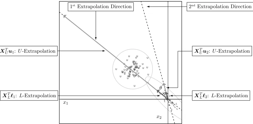
Figure 2: The dashed lines are the 1stand 2nd extrapolation directions for the block extrap-olation example from Figure 1. The extent ofU-extrapolation vector is a larger multiple of the extent ofL-extrapolation vector in the 1stversus the 2nd extrapo-lation direction, so predictions corresponding to feature vectors on the 1st extrap-olation direction are shrunk more than those on the 2nd extrapolation direction under the proposed method.
supervised linear regression estimator) is not unique since rank(XL) = 1, but the semi-supervised estimatorβb = XTL1YL/2
~
1 is the unique solution to
min
β kYL−XLβk
2
2+kXUβk22. (1)
Thisβb is the ordinary least squares estimator with equal components, so it achieves objec-tives (i) XLβb =XLβb
(OLS)
and (ii)XUβb = XTL1YL/2
XU~1 =~0. Optimization Problem (1) is a special case of the joint training framework to come in Section 3, and our general semi-supervised approach is based on this type of estimator.
Block Extrapolation Example: These data in Figure 2 include two lines marked as 1st and 2nd extrapolation directions, and each direction has extent vectors of largest U -and L-extrapolations (XTL`1, XTUu1 and XTL`2, XTUu2). Each L-based extent vector in Figure 2 is the longest possible of the formXTL`in a given direction for`∈IR|L|such that
k`k22 = 1. Similarly, theU-based extent vectors are the longest possible in a given direction based on a unit length linear combination of the rows of XU. While precise mathematics on determining the two extrapolation directions is deferred until Section 4, it also turns out that the ratio ofU- toL-extent vector lengths in the 2nd direction is never bigger than that in the 1st direction, i.e.,
XTUu2
2
XTL`2 2
≤
XTUu1
2
XTL`1 2
The sought after compromise is struck with semi-supervised estimator βb by shrinking a supervised estimator βb
(SUP)
with respect to a basis of directions orthogonal to the extrapo-lation directions. With this in mind, define the decomposition of a supervised estimate
b
β(SUP)= ˜ν1+ ˜ν2, where ˜
ν1 is orthogonal to the 1stextrapolation direction (3) ˜
ν2 is orthogonal to the 2nd extrapolation direction, and consider a semi-supervised estimate of the form
b
β=p1ν˜1+p2ν˜2, wherep1 =
XTL`1
2
XTL`1
2+ XTUu1
2
and p2 =
XTL`2
2
XTL`2
2+ XTUu2
2
. (4)
Coefficient shrinking is more focused on the vector orthogonal to the 1st extrapolation direction because 0≤p1 ≤p2 ≤1 by Inequality (2).
A semi-supervisedβbfrom Display (4) was decomposed with regard to a basis orthogonal to directions of extrapolations from Display (3) so that linear predictions xT0βb at an arbi-trary feature vectorx0 ∈IR2 are shrunk more heavily when x0 is in directions with larger extrapolations. To demonstrate this, define a closely related decomposition of a feature vector
x0 =ν1+ν2, where
ν1 is on the 1st extrapolation direction (5)
ν2 is on the 2nd extrapolation direction.
Together, Decompositions (4) and (5) result in the semi-supervised prediction
x0Tβb =p1νT1ν˜2+p2νT2ν˜1
becauseνT1ν˜1=ν2Tν˜2= 0 by construction. Thus, with fixed length feature vectorsx0 =νi on the 1stand 2ndextrapolation directions, the 1stdirection corresponds to a semi-supervised predictionxT0βbthat is a more heavily shrunken version of its supervised predictionxT0βb
(SUP)
whenever p1 < p2.
The supervised estimate βb = βb (SUP)
results whenever p1 = p2 = 1, by Displays (3) and (4). Thus, supervised predictions are favored when L-based extrapolations XTL`i
2 dominate U-based extrapolations XTUui
2 because pi ≈1 follows from Display (4). On the other hand, predictions near zero are favored when U-based extrapolations dominate
L-based extrapolations (pi ≈0). In both cases, thepi regulate the compromise (i) with (ii) forβb term-by-term in each extrapolation direction. A significant contribution of this work is to provide a rigorous mathematical framework to study semi-supervised linear predictions for unlabeled extrapolations. In Section 4, directions of extrapolation and relative degrees of shrinkingpi are shown to follow from the joint trained optimization framework.
2.2 Model-based Contributions of Unlabeled Data
Under the linear model (E[Y] =Xβ and Var(Y) =σ2I), the coefficient parameter space
data manifold and on the model parameterσ2. The general theme is that lucky (unlucky)
β’s are in directions orthogonal (parallel) to the unlabeled feature data manifold, so lower variability within this manifold implies more lucky β directions where our approach im-proves performance. A general bound is presented in Section 5 to help understand when our semi-supervised linear adjustment is guaranteed to outperform its supervised baseline on unlabeled predictions. Next, the collinearity and block extrapolation examples from Section 2.1 are revisited to illustrate lucky versus unlucky (or favorable versus unfavorable) prediction scenarios.
Collinearity Example: This example hadp= 2,XL1=XL2, and XU1=−XU2. A lucky β follows with β= (b, b)T for some arbitrary b∈IR, since XUβ =~0 is clearly ideal for the semi-supervised approach. On the other hand, suppose the true β = (b,−b)T for some scalar b of large magnitude, and the components of XU1 are all of large magnitude with the same sign. This is an example of an unlucky β since the truthXUβ= 2bXU1 is far from the origin~0 with components of the same sign, so setting XUβb =~0 is less than ideal. SinceXLβ=~0, the typical supervised linear regression estimators (e.g., ridge, lasso, and ENET) would predict theXU cases close to~0 not 2bXU1 and does not fair much better as a result. The bottom-line is that this unlucky β situation is not handled well by the conventional wisdom in machine learning of shrinking to optimize the bias-variance tradeoff (Hastie et al., 2009).
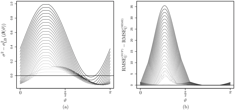
Block Extrapolation Example: This example was the block extrapolation from Figures 1 and 2. As it turns out, the ridge regression version of the Section 5 bound simplifies to a function of justβ (call itσLB2 (β)) such that the semi-supervised approach is guaranteed to outperform the supervised approach whenever σ2 −σ2
LB(β) >0 at a given
σ2. Next, this bound is used to give a snapshot of parameter space (β, σ2) in the context of the block extrapolation example, where lucky β correspond to σ2 −σLB2 (β) > 0 while unluckyβ correspond to σ2−σ2
LB(β)≤0.
In order to investigate this, take all σ2∈[0,1] with all possible coefficient vectors
β(ϑ) =
sin(ϑ) cos(ϑ)
forϑ∈[0, π]
0.0
0.2
0.4
0.6
0.8
1.0
π
2 π
0
ϑ
σ
2−
σ
2 LB
(
β
(
ϑ
))
(a)
0
5
10
15
20
25
30
35
π
2 π
0
ϑ
RMSE
(SUP) U
−
RMSE
(SEMI) U
(b)
Figure 3: (a) The theoretical bound σ2 −σLB2 (β(ϑ)) is plotted against ϑ for the block extrapolation example from Figures 1 and 2. Darker curves correspond to larger
σ2. Interest was in identifying ϑ such that σ2 −σ2LB(β(ϑ)) > 0, since values greater than zero highlight the lucky unit length directions β(ϑ) at a given σ2
where our semi-supervised adjustment helps. (b) The corresponding differences between supervised and semi-supervised root mean squared errors (RMSEs) on the unlabeled set are displayed.
In general, the proposed approach is well suited for lucky βprediction problems, which include the following generalization of the Figure 1 block extrapolation example. The distance between feature data centroids (i.e., between the originXTL~1/|L|=~0 due to mean centering and XTU~1/|U|) is increased relative to the variation about each centroid and the true coefficient vectorβis not roughly a multiple ofXTU~1/|U|. One might conjecture lucky
β to occur more often in practice during high-dimensional applications with large p by a sparsity of effects assumption (i.e., the trueβhas few non-zero components). For example, if the unlabeled feature data are concentrated on a low dimensional manifold away from the labeled data, there are more lucky directions for the true coefficient vector to emphasize directions away from the unlabeled feature data manifold. Also note that the supervised RMSEs are no better than semi-supervised in the block example, i.e., no negative differences in Figure 3(b). In theory, our technique handles unlucky β by defaulting to supervised predictions; see Remark 1 for how unlucky scenarios are handled empirically in practice.
directions in the unlabeled data, but there is no guarantee here either (i.e., the supervised technique may still perform much worse). In this work, we do not assume that the response is generated under a lucky β linear model. Instead, a tuning parameter is used to move the semi-supervised estimator closer to supervised in such cases to mitigate the losses relative to supervised for an unlucky β. Cross-validation is used to estimate this parameter in the results Section 6.
3. A Linear Joint Training Framework
The focus of this paper is the joint trained elastic net
b
αγ,λ,βbγ,λ
= arg min α,β
kYL−XLβk22+γ1kXU(α−β)k22+γ1γ2kαk22+λ1kβk11+λ2kβk22, (6)
whereβbγ,λis appropriately scaled andλ= (λ1, λ2)∈[0,∞]2and γ= (γ1, γ2)∈[0,∞]2 are tuning parameter vectors. The joint trained elastic net is an example of a joint training opti-mization framework used in semi-supervised learning (Chapelle et al., 2006b). Comparisons will be made to thesupervised optimization
b
β(ENET)λ = arg min
β
kYL−XLβk22+λ1kβk11+λ2kβk22, (7) which is a partial solution to Joint Optimization (6) wheneverγ1 = 0 orγ2 = 0.
Let XUXTU =OUDUOUT be the eigendecomposition of this outer product and define
X(γ2) = XL
X(γ2) U
!
= √ XL
γ2(DU+γ2I)−
1
2OTUXU !
(8)
forγ2>0. Proposition 2 establishes that the reduced problem b
βγ,λ= arg min
β
kYL−XLβk22+γ1 X
(γ2) U β
2
2+λ1kβk 1
1+λ2kβk 2
2 (9)
is an alternative to Joint Optimization (6) over (α,β)∈IRp×IRp.
Proposition 2 If γ2 > 0, then rank(XU) = rank
X(γ2) U
and a solution βbγ,λ to
Opti-mization Problem (9) is a partial solution to OptiOpti-mization Problem (6).
By Proposition 2, the semi-supervised estimate βbγ,λ can be computed by an elastic net subroutine through data augmentation if the user simply inputs the supervised tuning parameters λ with model matrix
XTL, √γ1X(γU2) TT
and response vector
YTL, ~0TT (i.e., impute YU =~0). The Elastic Net Optimization Problem (7) is convex and can be solved quickly by theglmnet package inR(Friedman et al., 2010; R Core Team, 2015), so this helps make our semi-supervised adjustment computationally viable.
MatrixX(γ2) U
T
X(γ2)
U from Optimization Problem (9) has the same eigenvectors asX T UXU, but its eigenvalues homogenize to unity as γ2 → 0. As γ2 → ∞,X(γU2)
T
X(γ2)
U → XTUXU, and Optimization Problem (9) goes to thesemi-supervised extreme
b
β(γ1,∞),λ= arg min β
kYL−XLβk22+γ1kXUβk22+λ1kβk 1
1+λ2kβk 2
Semi-Supervised Extreme (10) with λ = ~0 and γ1 = 1 was seen earlier in Problem (1) during the conceptual overview. Finite γ2 > 0 will later be seen to produce intermediate compromises between Supervised (7) and Semi-Supervised Extreme (10).
4. Geometry of Semi-Supervised Linear Regression
A geometrical understanding of the Joint Trained Elastic Net (6) is developed through the following logical progression: Section 4.1 joint trained least squaresλ=~0, Section 4.2 joint trained ridge λ = (0, λ2), Section 4.3 joint trained lasso λ= (λ1,0), and then Section 4.4 joint trained elastic net regression λ. Last, Section 4.5 provides a gallery of geometrical examples. The conceptual overview from Section 2.1 lines-up closely with the mathematics of Section 4.1 and is back-referenced extensively to help the reader make connections. The ridge, lasso, and elastic net semi-supervised geometries do, to some degree, simply follow from their well-known supervised properties when combined with the geometrical properties of joint trained (semi-supervised) least squares. However, an important subtlety is worth mentioning. This geometry section, especially Sections 4.3 and 4.4, establishes properties of the Joint Trained Elastic Net (6), and these properties are stated as the assumptions of Section 5 in order to derive general performance bounds that necessarily apply to the joint trained elastic net.
4.1 Joint Trained Least Squares
Optimization Problem (9) withλ=~0 reduces tojoint trained least squares
b
βγ = arg min
β
kYL−XLβk22+γ1 X
(γ2) U β
2
2. (11)
Briefly recall the collinearity example from Section 2.1, i.e., p = 2, XL1 = XL2, XU1 =
−XU2, and γ = (1,∞). A supervised βb (OLS)
was not unique, but the βb (OLS)
with equal components was the unique semi-supervised Estimator (11). In general, Estimator (11) is unique whenever γ > ~0 and rank(X) = p. Henceforth, assume rank(XL) = p, so b
β(OLS) = XTLXL −1
XTLYLis unique during this discussion of joint trained least squares. Section 4.2 on joint trained ridge regression is tailored for rank(XL)< p.
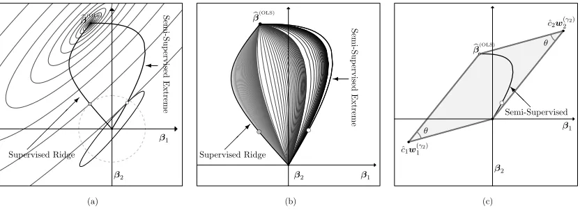
Figure 4(a) displays the semi-supervised extreme βbγ
1,∞ from the block extrapolation example for a particular γ1 > 0 based on the calculus of Lagrangian multipliers. For generalp≥2 with γ2≥0, there exists unique scalarsaγ2, bγ2 such that the ellipsoids
βTX(γ2) U
T
X(γ2)
U β ≤ aγ2 (12)
β−βb (OLS)T
XTLXL
β−βb (OLS)
≥ bγ2 (13)
have the same tangent slope at the point of intersectionβbγ. A novelty of the semi-supervised approach, that holds for generalp≥2, is the use of origin-centered Ellipsoids (12) as opposed to the multidimensional spheres used in supervised ridge regression.
When γ2 ≈ 0, βbγ ≈ βb (RIDGE)
γ1 = X
T
LXL+γ1I −1
● ●
● ●
●
● ●
β2
β1
b
β(OLS) Semi-Sup
ervised
Extreme
Supervised Ridge
(a)
● ●
● ●
●
● ●
(b)
β2 β1
Semi-Sup
ervised
Extreme
b
β(OLS)
Supervised Ridge
●
●
●
●
● ●
● ●
(c)
β1
β2
b
β(OLS)
ˆ
c2w(2γ2)
ˆ
c1w (γ2) 1
θ
θ
Semi-Supervised@
@ I
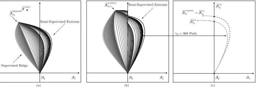
Figure 4: The Figure 1 block example is revisited. (a) A labeled responseYL that resulted in the plotted estimate βb
(OLS)
is part of the assumed labeled data set. Each estimate on the semi-supervised extreme βbγ
1,∞, like the small white circle at
γ1 = 0.18, is the intersection of an origin-center Ellipse (12) and aβb (OLS)
-centered Ellipse (13) having the same tangent slope at this point of intersection. Similarly, each ridge estimate, like the small gray circle withλ2= 5.9, uses origin-centered, concentric circles instead of Ellipses (12). (b) Paths βbγ varying γ1 with darker curves for largerγ2 fill-in all possible compromises between supervised ridge and the semi-supervised extreme. (c) The semi-supervised extreme βbγ
1,∞ is shrunk within its bounding parallelogram from supervised βb
(OLS)
toward the origin as
γ1 → ∞.
extreme. For example, take the point along the supervised ridge (semi-supervised extreme) path indicated by the small gray (white) circle in Figure 4. Paths βbγ, like those in Figure 4(b), start atβb
(OLS)
and converge to a point in the null space of XU as γ1 → ∞. The semi-supervised estimator for anyγ is
b
βγ =
XTLXL+γ1X(γU2) T
X(γ2) U
−1
XTLXLβb (OLS)
= I+γ1M(γ2) −1
b
β(OLS), where M(γ2)= XT LXL
−1
X(γ2) U
T
X(γ2) U .
(14)
An eigenbasis n
w(γ2) i , τ
(γ2) i
op
i=1 ofM
(γ2) such that XLw
(γ2) i
2
2 = 1 will be used to help understand how joint trained least squares regression coefficients are shrunk. Proposition 3 establishes that this important eigenbasis is real whether or not matrixM(γ2) is symmetric.
Proposition 3 Any eigenbasis of the possibly non-symmetric matrix M(γ2) is real with
eigenvalues τ(γ2)
1 ≥ · · · ≥τ (γ2)
p ≥0. Furthermore, τi(γ2)= 0 iff i >rank(XU). While nw(γ2)
i op
i=1 may be neither orthogonal nor unit length,
b
β(OLS) = ˆc(γ2)
1 w
(γ2)
1 +· · ·+ ˆc (γ2)
for some scalars ˆc(γ2)
i , and by Equations (14) and (15),
b
βγ = 1
1 +γ1τ1(γ2) !
ˆ
c(γ2)
1 w
(γ2)
1 +· · ·+
1 1 +γ1τp(γ2)
! ˆ
c(γ2)
p w(γp 2). (16) Equations (15) and (16) generalize Estimator (4) from Section 2.1 to p ≥ 2. The terms on the right of Equation (15) were previously denoted by the ˜νi from Display (3), and these terms are weighted by proportions on the right of Equation (16) that were previously denoted by the pi from Display (4). Eigenvector ˆc(γ1 2)w
(γ2)
1 is proportionally shrunk the most at any fixed γ1 >0 because its proportion weight 1/
1 +γ1τ1(γ2)
is the smallest. The bounding parallelogram in Figure 4(c) helps introduce another interpretation of Equation (16). This parallelogram has opposite corners at the origin and βb
(OLS)
and sides parallel to the eigenvectors ofM(γ2). The path
b
βγ shrinks fromβb (OLS)
to the origin along the sides with corner ˆc(γ2)
2 w
(γ2)
2 asγ1 ∈[0,∞] increases and does so more closely whenτ1(γ2) and τ(γ2)
2 differ in magnitude. Proposition 4 generalizes this concept to arbitrary γ2 ≥ 0 and p≥2.
Proposition 4 The path βbγ as a function of γ1 ≥ 0 is bounded within a p-dimensional
parallelotope with corners at each binary linear combination ofnˆc(γ2)
1 w
(γ2) 1 , . . . ,ˆc
(γ2) p w(γp2)
o
.
Furthermore, the terminal point as γ1 → ∞ is the cornerPpi=1I{i>rank(XU)}ˆc
(γ2)
i w
(γ2) i with
indicator I{·}.
The conceptual overview in Section 2.1 made a careful distinction between shrinking re-gression coefficientsβb versus shrinking linear predictionsxT0βb. Vectors ˜νi from Display (3) were related to coefficient shrinking, whereas νi from Display (5) were the feature vectors
x0 related to prediction shrinking. Mathematically, eigenvectorsw(γi 2)determine directions of coefficient shrinking. Since p = 2, the Section 2.1 discussion in-fact concentrated on all feature vectors w(γ2)
1 ⊥
and w(γ2) 2
⊥
, and an eigenvector direction of maximum (minimum) coefficient shrinking was orthogonal to feature vectors of maximum (minimum) prediction shrinking. Generalizing this story top >2 also results inpdirections of coefficient shrinking and p feature vector directions of interpretable prediction shrinking, but the mathematics has the following subtlety. Whenp >2, a direction of coefficient shrinking w(γ2)
i is orthog-onal to a p−1 dimensional vector space w(γ2)
i ⊥
of feature vectors, so if p−1≥2, vector space w(γ2)
1 ⊥
consists of an infinite number of directions. Proposition 5 below provides a convenient form for the line in common to allw(γ2)
j ⊥
withj6=ifor eachi∈ {1, . . . , p}by es-tablishing a relationship betweenw(γ2)
i ,w (γ2) i
⊥
, andX(γ2)from Equation (8). Theseplines of feature data vectors for arbitrary p≥2 will later be seen to have a clear interpretation when it comes to prediction shrinking, so we call them extrapolation directions.
Proposition 5 The span
X(γ2)TX(γ2)w(γ2) i
= T
j∈{1,...,p}−{i}w (γ2) j
⊥
∀i ∈ {1, . . . , p}. Henceforth, the line span
X(γ2)TX(γ2)w(γ2) i
is called the ith extrapolation direction ∀i∈
The ith extrapolation direction necessarily traces out a line because it’s all scalar mul-tiples of the nonzero vectorX(γ2)TX(γ2)w(γ2)
i . Any feature vector on the i
th extrapolation
direction, i.e., x0 ∈ Tj∈{1,...,p}−{i}w (γ2) j
⊥
from Proposition 5, is of special note. Their Equation (16) semi-supervised predictions simplify toxT0βbγ = ˆc
(γ2) i /
1 +γ1τi(γ2)
xT0w(γ2) i
and are shrunk more (relative to the corresponding OLS supervised prediction xT0βb (OLS)
= ˆ
c(γ2) i xT0w
(γ2)
i ) for smalleri∈ {1, . . . , p}at any fixed γ1 >0 becauseτ1(γ2)≥ · · · ≥τ (γ2) p . Next, the ith extrapolation direction is shown to be one of more (or less) extreme un-labeled extrapolations. With this in mind, use the indicator function I{·} to define the positive numberκ(γ2)
i =τ (γ2)
i +I{i>rank(XU)} and define the vectors
`(γ2)
i =XLw(γi 2) and u (γ2)
i =
X(γ2)
U w
(γ2) i q
κ(γ2) i
. (17)
Vectors (17) in the semi-supervised extreme ofγ2 =∞were temporarily denoted by`i and
ui during their more conceptual introduction within Section 2.1 (e.g., Figure 2). It was also stated previously during this overview that `i and ui were unit length. Proposition 6 is a generalization.
Proposition 6 If γ2 > 0, vectors n
`(γ2) i
o1
i=p and n
u(γ2) i
orank(XU)
i=1 are orthonormal bases
for the column spaces ofXL and X(γU2), and ui(γ2)=~0 if i >rank(XU).
Section 2.1 also introduced extents of L- andU-extrapolation. Vectors (17) are used to define these now for eachi∈ {1, . . . , p}as
XTL`(γ2)
i Extent of L-Extrapolation (in the i th
Direction)
X(γ2) U
T
u(γ2)
i Extent of U-Extrapolation (in thei th
Direction), where (18) spanX(γ2)TX(γ2)w(γ2)
i
is the ith Direction of Extrapolation from Proposition 5.
Propositions 7 establishes that the ith extent vectors are in-fact on the ith extrapolation direction.
Proposition 7 For each i∈ {1, . . . , p},
XTL`(γ2)
i =
1 1 +τ(γ2)
i
X(γ2)TX(γ2)w(γ2) i
X(γ2) U
T
u(γ2)
i =
τ(γ2) i
(1 +τ(γ2) i )
q
κ(γ2) i
X(γ2)TX(γ2)w(γ2) i ,
so X(γ2)TX(γ2)w(γ2) i ,XTL`
(γ2)
i , and X
(γ2) U
T
u(γ2)
Previously defined vectors are now verified to possess fundamental interpretations: (i) Extent Vectors (18) do indeed measure “extrapolation extents” in a sensible manner, (ii) Vectors (17) determine shrinking directions for joint trained least squares fits Xβbγ, and (iii) magnitudes of extent vectors regulate the shrinking of regression coefficientsβbγ. These three interpretations are gleaned by applying Propositions 6 and 7 in conjunction with well-known properties of orthogonal projection matrices and quadratic forms from linear algebra. Then×p matrix identity
X(γ2)
w(γ2)
1 · · · w (γ2) p
=
`(γ2) 1 q
κ(γ2) 1 u
(γ2) 1
!
· · · `
(γ2) p q
κ(γ2) p u(γp2)
!!
(19)
follows from Definitions (17). The right of Equation (19) has orthogonal columns by Propo-sition 6, and the columns on the left of Equation (19) are eigenvectors with eigenvalue one of the orthogonal projection matrix X(γ2)
X(γ2)TX(γ2) −1
X(γ2)T. Therefore, the columns of Matrix (19) are an orthogonal basis for the eigenspace ofX(γ2)
X(γ2)TX(γ2) −1
X(γ2)T corresponding to eigenvalue one, because rankX(γ2)
=pis a necessary condition for the joint trained least squares assumption that rank(XL) =p.
Projection matrix X(γ2)
X(γ2)TX(γ2) −1
X(γ2)T is nonnegative definite, so its main diagonal block sub matrices based on theL,U data partition are also nonnegative definite. The nonnegative definite, rank-p, sub matrix XL
X(γ2)TX(γ2) −1
XTL has orthonormal
eigenvectors n`(γ2) i
o1
i=p corresponding to its nonzero eigenvalues 1/(1 +τ (γ2)
i ) by Proposi-tions 6 and 7. Similarly, nonnegative definite sub matrix X(γ2)
U
X(γ2)TX(γ2) −1
X(γ2) U
T
has orthonormal eigenvectors nu(γ2) i
orank(XU)
i=1 corresponding to its nonzero eigenvalues
τ(γ2) i /(1+τ
(γ2)
i ). Well-known eigenvector solutions to constrained optimizations of quadratic forms imply
`(γ2)
i = arg max
υ∈IR|L|:υTυ=1,υT`(γ2)
j =0 ∀j>i
υTXL
X(γ2)TX(γ2) −1
XTLυ
u(γ2)
i = arg max
υ∈IR|U|:υTυ=1,υTu(γ2)
j =0 ∀j<i
υTX(γ2) U
X(γ2)TX(γ2) −1
X(γ2) U
T
υ.
In other words, the unit length weight vectors on the rows ofXL(ofX(γU2)) that maximize a Mahalanobis distance measuring extent of extrapolation subject to orthogonality constraints are the eigenvectorsn`(γ2)
i o1
i=p(eigenvectors n
u(γ2) i
orank(XU)
i=1 ) sorted by descending positive eigenvalues. Proposition 7 also establishes that each eigenvalue
τ(γ2)
i =
X(γ2) U
T
u(γ2) i
2
X
T L`
(γ2) i
2
of the shrinking matrix M(γ2) from Display (14) is a ratio of parallel extent eigenvector lengths, so the extent ofU-extrapolation is larger (smaller) than the correspondingL-extent in theith direction of extrapolation if τ(γ2)
i >1 (ifτ (γ2) i <1).
The joint trained least squares fits vector for all nobservations has the form
Xβbγ = p X
i=1 ˆ
c(γ2) i
1 1 +γ1τi(γ2)
!
`(γ2) i q
κ(γ2)
i /γ2OU(DU+γ2I) 1 2u(γ2)
i !
by Equations (16) and (19) and the reverse of Transformation (8). Thus, eigenvectors`(γ2) i andu(γ2)
i involved in constructing thei
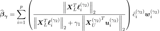
th extrapolation direction with smalleri∈ {1, . . . , p} are used to shrink fits more asγ1 is increased. By Equation (16) and Ratios (20), coefficient vector
b
βγ = p X
i=1
X
T L`
(γ2) i
2
X
T L`
(γ2) i
2+γ1
X(γ2) U
T
u(γ2) i
2
ˆ
c(γ2)
i w
(γ2) i
is a generalization of Display (4) and balances the degree of coefficient shrinkage by the relative extents ofU- versusL-extrapolations in theith direction as tuning parameter γ
1 is increased.
The Figure 2 block extrapolation example is now revisited with the notation of Display (18) and other mathematical developments from this section in mind. Extrapolation di-rections can always be computed with Proposition 5. When p = 2, the 1st extrapolation direction is comprised of all vectors orthogonal tow(γ2)
2 , and the 2
ndextrapolation direction is comprised of all vectors orthogonal to w(γ2)
1 . Directions and extents in Figure 2 were all based on the semi-supervised extreme setting γ2 = ∞. In this example, the extent of
U-extrapolation is a larger multiple of theL-extent in the 1st direction, soτ(γ2)
1 > τ
(γ2) 2 is a strict inequality. In addition,U-extents have the larger magnitude, so τ(γ2)
2 >1 is another artifact of this particular example. An example of p > 2 is deferred until discussion of Figure 6 in the examples Section 4.5.
4.2 Joint Trained Ridge Regression
Estimator (9) withλ= (0, λ2) is motivated with augmented labeled data
X(λ2)
L =
XL
√
λ2I
and Y?L=
YL
~0
(21)
having padditional rows. The resulting joint trained ridge estimator
b
βγ,(0,λ2)= arg min
β
kYL−XLβk22+γ1 X
(γ2) U β
2
2+λ2kβk 2 2 is equivalent to Joint Trained Least Squares (11) given Data (21). Hence,
b
βγ,(0,λ2) =
X(λ2) L
T
X(λ2)
L +γ1X (γ2) U
T
X(γ2) U
−1
X(λ2) L
T
X(λ2) L
b
● ●
● ●
● ●
β2 β1
b β(OLS)
Semi-Supervised Extreme
Supervised Ridge
b β(RIDGE)λ2
@ @ R
(a)
● ●
● ●
β2 β1
b
β(LASSO)λ1 Semi-Supervised Extreme
@ R
(b)
γ2= 308 Path
-● ●
● ●
● ●
● ●
(c)
b β(LASSO)λ1 =βb
[j1]
λ1
b β[j3]
λ1
b β[j2]
λ1
r r
β2 β1
Figure 5: Paths of candidate βbγ,λ for the Figure 1 block example varying γ1 > 0 with darker curves for larger γ2 > 0 are compared. (a) Joint trained ridge paths at a fixedλ = (0,0.1) start at supervised ridge βb
(RIDGE)
λ2 instead of supervised OLS b
β(OLS). (b) Similarly, joint trained lasso paths at a fixed λ = (0.01,0) start at supervised lassoβb
(LASSO)
λ1 . However, these continuous paths are not differentiable at points where the active set changes. (c) The path from (b) with γ2 = 308 is highlighted. Active set changes are marked by bullets •, and the reference curves based on the right of Equation (23) are also displayed as dashed lines for
i = 1,2,3. Each reference curve starts at a βb [ji]
λ1 (marked by an open circle ◦) and terminates at the origin. The actual candidate path always equals one of the displayed reference curves. It starts atβb
(LASSO) λ1 =βb
[j1]
λ1 when γ1 = 0 and switches reference curves whenever there is a change in the active set.
becauseβb (RIDGE)
λ2 =
X(λ2) L
T
X(λ2) L
−1
XTLYLis the OLS estimator given Data (21). Matrix
X(λ2) L
T
X(λ2)
L = XTLXL+λ2I with λ2 > 0 is positive definite, so the inverse required to compute βbγ,(0,λ
2) exists. Estimates (22) for the block extrapolation example come out as expected in Figure 5(a). Paths start atβb
(RIDGE)
λ2 with λ2 = 0.1 and converge to the origin.
4.3 Joint Trained Lasso Regression
Supervised Optimization (7) withλ2= 0 simplifies toβb (LASSO) λ1 =βb
(ENET)
λ1,0 , a well-understood technique for incorporating variable selection when p is large and the columns of XL are linearly independent (Friedman et al., 2010). The goal in this section is to use what is already known aboutβb
(LASSO)
λ1 to provide an understanding of thejoint trained lassoβbγ,(λ1,0) from Problem (9). Denote the active set of some estimate βb by A ⊂ {1, . . . , p}, so
b
β
A is its|A| ×1 vector of nonzero components andβb
¯ A=
~0 is (p− |A|)×1. Also denote its
sign vector by s= sign
b
β
A
active set columns by XLA. The active setA(SUP) and sign vectors(SUP) of the supervised lasso at a given λ1 satisfy the constraint
XTLA(SUP)XLA(SUP)
b
β(LASSO)λ1
A(SUP) =X T
LA(SUP)YL−λ1s (SUP)
.
Estimates βb (LASSO)
λ1 are a differentiable function in λ1 with a finite number of exceptions. This function is continuous, but not differentiable when the active set changes.
The joint trained lasso βbγ,(λ
1,0) has properties similar to the supervised lasso by Opti-mization (9), because it’s a lasso estimator with unlabeled imputationsYU =~0 and modified
X. Unlike joint trained ridge and joint trained least squares from Sections 4.1 and 4.2, the joint trained lasso coefficients are not always a linear combination of the supervised lasso, and this complicates its ensuing interpretation. There are 2p+ 2p+ 1 active-set/sign-vector combinations for any p ≥2. For example, when p = 2, there are nine combinations, i.e., 22 = 4 quadrants, 2×2 = 4 axial directions, and 1 origin. Each active-set/sign-vector com-bination has a set of reference coefficients
b
β[λj1]
Aj
=
XTLAjXLAj
−1
XTLAjYL−λ1sj
and βb [j] λ1
¯ Aj
=~0 for j = 1, . . . ,2p + 2p+ 1. These reference coefficients have important
properties. First,βb [j]
λ1 are independent ofXU. Second, there exists aj∈ {1, . . . ,2
p+ 2p+ 1}
such that βb (LASSO) λ1 =βb
[j]
λ1. Third, sign
b
β[λj1]
Aj
does not necessarily equalsj. Next, the path of the joint trained lasso as a function of γ1 at a given γ2 is studied. Let the finite set
{ai}ki=1 be the finite values ofγ1 where the active set of the joint trained lasso changes and define a0 = 0 and ak+1 =∞. Also define the subsequence j1, . . . , jk such that Aji and sji
correspond to the joint trained lasso for any γ1 ∈[ai−1, ai), so this subsequence tracks the evolution of the joint trained lasso’s active set and sign vector. Thus, for allγ1∈[ai−1, ai),
b
βγ,(λ1,0)
Aji =
XTLA
jiXLAji+γ1X
(γ2)T UAjiX
(γ2) UAji
−1
XTLA
jiXLAji
b
β[jλ1i]
Aji, (23) and shrinking of regression coefficients on the active set looks very much like Display (14).
i 1 2 3 4
Aji {1,2} {2} {1,2} ∅ sTji (−1,1) (0,1) (1,1)
-γ1 [0,0.004) [0.004,0.008) [0.008,∞) ∞
Table 1: Block extrapolation active-set, sign-vector combinations are listed as a function of
γ1 for the joint trained lasso coefficients βbγ,λ from Figure 5(c) with λ= (0.01,0) and γ2 = 308.
Figure 5(b) plots paths of vectors βbγ,(λ
1,0) byγ2 as a function ofγ1 atλ1= 0.01 for the block extrapolation example. The semi-supervised path starts at the supervised estimate b
small regionγ1 ∈[0, a1), wherea1>0. This local property of the joint trained lasso, which was mathematically verified in this section, is stated as a key assumption while deriving the general performance bounds in Section 5. An example is the highlighted path withγ2= 308 from Figure 5(b) shown in Figure 5(c). This candidate path of semi-supervised regression coefficients visits four active-set, sign-vector combinations as a continuous function of γ1 at given λ1 and γ2. These visited combinations are listed in Table 1 along with their corresponding valuesγ1. Figure 5(c) also includes dashed reference curves based on the right of Equation (23) as a function ofγ1 for each non-empty active-set/sign-vector combination visited by the approach, i.e., i = 1,2,3. The candidate semi-supervised estimates follow along a reference path until the active set changes, and then the path switches to the reference path with the new active set and sign vector. This continues until the path terminates at the origin whenγ1=∞.
4.4 Joint Trained Elastic Net Regression
A general view of Problem (9) when all four tuning parameters are finite and positive comes from stringing concepts from Sections 4.2 and 4.3 together. In particular,
b
βγ,λ
Aji =
X(λ2) LAji
T
X(λ2)
LAji +γ1X(γUA2)ji T
X(γ2) UAji
−1
X(λ2) LAji
T
X(λ2) LAji
b
β[λji]
Aji,
whereAji and sji depend on (γ,λ) and
b
β[λji]
Aji = (1 +λ2)
X(λ2) LAji
T
X(λ2) LAji
−1
X(λ2)T
LAjiYL−λ1sji
.
The order of operations are important: substituteXLAji forXLand then apply Equation (21) to get X(λ2)
LAji, and similarly, XUAji for XU to then get X(γUA2)ji from Equation (8). Increased γ1 and γ2 puts more emphasis on shrinking unlabeled fits. Increasedλ2 and/or decreasedγ2results in the labeled and/or unlabeled directions being better approximated by an |Aji|-sphere, and increased λ1 for presumably more stringent variable selection. Cross-validation often selects the joint trained elastic net with strictly positive lasso λ1 >0 and ridgeλ2 >0 tuning parameter values in practical applications, so the joint trained elastic net is showcased later through its performance on numerical examples (i.e., simulated and real data sets) in Section 6.
4.5 Geometric Extrapolation Examples
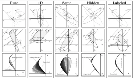
The purpose of this section is learn more about the properties of our semi-supervised adjust-ment through additional geometrical examples of joint trained least squares from Section 4.1. Recall the joint trained least squares example in Figures 1, 2, and 4 for the heav-ily studied block extrapolation example. The first row of Figure 6 motivates additional discussion by simply changing the unlabeled feature data as follows.
Pure ● ●● ● ● ● ● ● ● ● ● ●● ● ● ● ● ● ● ● ● ● ● ● ● ● ● ● ● ● ● ● ● ● ●●● ● ● ● ● ● ● ● ● ● ● ● ● ● ● ● ● ● ● ● ● ● ● ● ● ● ● ● ● ● ● ● ● ● ● ● ● ● ● ● ● ● ● ● ● ● ● ● ● ● ● ● ● ● ● ●● ● ● ● ● ● ● ● x1 x2 θ
w(2γ2) ⊥
@ @
@ R
w(γ2) 1 ⊥ ● ● ● ● ●● ● ● ˆ
c(γ2) 2 w(2γ2)
ˆ c( γ 2 ) 1 w ( γ 2 ) 1 β1 β2 b β(OLS) θ θ Semi-Supervised ● ● ● ● ●● ● Semi-Supervised Supervised β1 β2 1D ● ● ● ● ● ● ● ● ● ● ● ●● ● ● ● ● ● ● ● ● ● ● ● ● ● ● ● ● ● ● ● ● ● ●● ● ●● ● ● ● ● ● ● ● ● ● ● ● ● ●● ● ● ● ● ● ● ● ● ● ● ● ●● ● ● ● ● ● ● ● ● ● ● ● ● ● ● ● ● ● ● ● ● ● ● ●● ● ● ● ● ● ● ● ● ● ● x1 x2 θ
w(2γ2) ⊥ w(γ2)
1 ⊥ ● ● ● ● ●● ● ● ˆ
c(2γ2)w (γ2) 2
ˆ
c(γ2) 1 w
(γ2) 1 β1 β2 b β(OLS) θ θ Semi-Supervised ● ● ● ● ●● ● Semi-Supervised @ @@R
Supervised β1 β2 Same ● ● ● ● ● ● ● ● ● ● ● ● ● ● ● ● ● ● ● ● ● ● ● ● ● ● ● ● ● ● ● ● ● ● ● ● ● ● ● ● ● ● ● ● ● ● ● ● ● ● ● ●● ● ● ● ● ● ● ● ● ● ● ● ● ● ● ● ● ● ● ● ● ● ● ● ● ● ● ● ● ● ● ● ● ● ● ● ● ● ● ● ● ● ● ● ● ● ● ● x1 x2 θ
w(2γ2) ⊥ w(1γ2)
⊥ ● ● ● ● ●● ● ● ˆ
c(γ2) 1 w
(γ2) 1 ˆ c( γ 2) 2 w ( γ 2) 2 β1 β2 b β(OLS) θ θ Semi-Supervised -● ● ● ● ●● ● Semi-Sup ervised Supervised β1 β2 Hidden ● ● ● ● ● ● ● ● ● ● ● ●● ● ● ● ● ● ● ● ● ● ● ● ● ● ● ● ● ● ● ● ● ● ● ●● ● ● ● ● ● ● ● ● ● ● ● ● ● ● ●● ● ● ● ● ● ● ● ● ● ● ● ● ● ● ● ● ● ● ● ● ● ● ● ● ● ● ● ● ● ● ● ● ● ● ● ● ● ● ●● ● ● ● ● ● ● ● x1 x2 θ
w(γ2) 2
⊥ w(1γ2)
⊥ ● ● ● ● ●● ● ● ˆ
c(γ2) 2 w
(γ2) 2
ˆ
c(γ2) 1 w
(γ2) 1 β1 β2 b β(OLS) θ θ Semi-Supervised ● ● ● ● ●● ● Semi-Supervised @ R Supervised β1 β2 Labeled ● ● ● ● ● ● ● ● ● ● ● ●● ● ● ● ● ● ● ● ● ● ● ● ● ● ● ● ● ● ● ● ● ●●●●●●● ● ● ● ●● ● ● ●●● ●●●●●● ●●● ● ● ● ●●●● ● ●●●● ●● ●● ● ● ●● ●●●●●● ●● ●●●● ● ●● ● ● ●● ● ● x1 x2 θ
w(γ2) 2
⊥ w(γ2)
1 ⊥ ● ● ● ● ●● ● ● ˆ
c(γ2) 2 w
(γ2) 2 ˆ c ( γ 2) 1 w ( γ 2) 1 β1 β2 b β(OLS) θ θ Semi-Supervised ● ● ● ● ●● ● Supervised Semi-Sup ervised β1 β2
Figure 6: An additional geometrical example of joint trained least squares is displayed in each column. Row 1: Only the unlabeled feature dataXU from the “working” block extrapolation example from Figures 1, 2, and 4 were changed. Row 2: Ellipses (12) and (13) intersect at a point on the semi-supervised extreme. Row 3: Pathsβbγ are plotted byγ2 varyingγ1. The gray circle is the supervised ridge solution from Figure 4(a).
• “1D” – The unlabeled marginal distribution is more volatile in one dimensionx2.
• “Same” – Minor discrepancies arise naturally in empirical distributions when taking independent samples from the same distribution.
• “Hidden” – Components x1 and x2 have roughly the same marginal distributions in both sets, but unlabeled extrapolations are hidden in the bivariate distribution of (x1, x2).
• “Labeled” – Only the labeled feature data deviate substantially from the origin.
Broader sets of candidate βbγ are entertained in the block, 1D, and same extrapola-tion examples. On the other hand, direcextrapola-tions of extrapolaextrapola-tions are roughly the principal components in the pure, hidden, and labeled extrapolation examples, and these exam-ples have smaller candidates sets βbγ as a result. In general, such smaller candidates sets are expected whenever the semi-supervised eigenvector directions of shrinking based on
XTLXL −1
X(γ2) U
T
X(γ2)
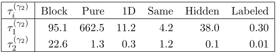
τ(γ2)
i Block Pure 1D Same Hidden Labeled
τ(γ2)
1 95.1 662.5 11.2 4.2 38.0 0.30
τ(γ2)
2 22.6 1.3 0.3 1.2 0.1 0.01
Table 2: The eigenvalues of M(γ2) with γ
2 =∞ are listed.
XTLXL, but this does not imply that supervised and semi-supervised ridge techniques are approximately the same (see Remark 8).
The block and pure examples emphasize profoundly different directions of extrapola-tion, but have eigenvalues of large magnitude in Table 2. Extrapolations are on separate manifolds, and the approach shrinks predictions much more in these two examples at a given γ1 >0, by Equation (16). The semi-supervised extreme path closely maps the sides of its bounding parallelogram from Proposition 4 in the pure and hidden examples because their τ(γ2)
i in Table 2 are of different orders of magnitude. This phenomena is not present in the block and same examples when eigenvalues are of the same order of magnitude. The semi-supervised extreme in the 1D example is of special note. Its labeled feature data are negatively correlated, so the extreme emphasizesx1to shrink the influence of the component
x2 which is volatile in the unlabeled data.
Figure 7 is a 3D example. In the semi-supervised extreme, the shrinking matrix M(γ2) has eigenvalues τ(γ2)
i = 2090,21.3,1.08, so shrinking of regression coefficients is much more heavily focused in directionw(γ2)
1 because these eigenvalues differ in magnitude. The 1st di-rection of extrapolation is based on the other p−1 = 2 directions of coefficient shrinking
w(γ2) 2 andw
(γ2)
3 and is defined as the set of all feature vectors that are orthogonal to both of these directions. The desired effect of using the unlabeled data to shrink unlabeled extrapo-lations more is achieved through Equation (16) at anyγ1>0. Semi-supervised predictions are xT0βb
(OLS)
/(1 +γ12090) if x0 is a feature vector on the 1st direction of extrapolation;
xT0βb (OLS)
/(1 +γ121.3) ifx0 is on the 2nd direction; andxT0βb (OLS)
/(1 +γ11.08) ifx0 is on the 3rddirection. Candidate vectors
b
βγ in Figure 7(b) form a curved surface between supervised and semi-supervised extreme.
Remark 8 Even if supervised and semi-supervised candidate sets βb are approximately
equal, semi-supervised training with the unlabeled feature data XU may pick a very
dif-ferent (and hopefully more advantageous) estimateβb within the candidate set during
cross-validation. In general, whether or not such apparent “parameter redundancies” exist, we always advocate the use of supervised regularization (λ 6=~0) together with semi-supervised regularization (γ 6=~0), especially when p is large. Many parameter redundancies noted in the p = 2 examples are not present in large p applications. If one briefly backs up to the case of p = 1, all candidate paths from Section 4.1 essentially start on the number line at the OLS estimate and then shrink to zero. When p = 3, one could overlay βbγ,(0,λ
2) for all
γ∈[0,∞]2 at fixedλ2 >0, and this in-fact adds a distinct layer to the 3D surface in Figure
L
L L
L L L
L
L L L LLL
L LL
L
L L
L
L
L L
L L
L L
L L
L L U
U U
U
U U
U U U
U
U
U U
U U
U U
U
U U
U
U
U U
U U U
U
U U
U
U UU
U
U
U U
U
U U U
U
U U
U U
U U U U
U U
U U
U U U
U U
U U
U U U
UU U
U
x3
x1
x2 1stExtrapolation Direction,w(γ2)
2 ⊥
∩w(γ2)
3 ⊥
H H
H HHj
2ndExtrapolation Direction,
w(γ2)
1 ⊥
∩w(γ2)
3 ⊥
3rdExtrapolation Direction,w(γ2)
1 ⊥
∩w(γ2)
2 ⊥
6 Labeled Data
Unlabeled Data
(a)
●
β3
β2
β1
b
β(OLS)
6
Semi-Supervised Extreme 6
Supervised Ridge
?
(b)
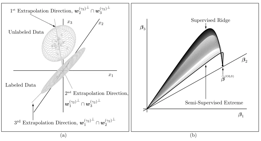
Figure 7: A p = 3 extrapolation data set is displayed. (a) The feature data along with the three extrapolation directions in the semi-supervised extreme ofγ2 =∞ are plotted. Each direction of extrapolation is a line that equals the intersection of two planes by Proposition 5. (b) Candidate paths βbγ by γ2 varying γ1 have a nonlinear compromise between supervised ridge and the semi-supervised extreme.
5. Performance Bounds
A general sufficient condition is given in this section for when a semi-supervised adjustment improves expected unlabeled prediction performance for a large class of linear supervised approaches. Assumption 1 on the class of supervised approaches is a necessary but not a sufficient condition for the elastic net; this generality was intentional. Assumption 2 characterizes a local property of our semi-supervised adjustment that follows from its Section 4 geometry.
Assumption 1: The supervised estimateβb
(SUP)
λ is unique for data(XL,YL) and some
λ. Letφ={λ,A,s} andq =|A| denote its fixed properties.
Assumption 2: ∃ δ > 0 such that ∀ γ1 ∈ [0, δ) semi-supervised estimates βb (φ) γ1 have
the supervised active setA and sign vectors, and
b
β(γφ1)
A =
I +γ1M(λ2, ∞) A
−1 b
β(SUP)λ
A, where
M(λ2,γ2)
A =
X(λ2) LA
T
X(λ2) LA
−1
X(γ2) UA
T
X(γ2) UA.
Assumptions 1 and 2 always hold for the Joint Trained Optimization Problem (6) when
Results to come focus on the impact of semi-supervised learning with γ2 = ∞, so Propositions 3-6 are applied toβb
(φ)
γ1 andM (λ2,∞)
A . Let n
w(iφ), τi(φ)oq
i=1be an eigenbasis of
M(λ2,∞)
A such that X
(λ2) LA w
(φ) i
2
2= 1 and
b
β(SUP)λ
A= Pq
i=1ˆc (φ) i w
(φ)
i generalize Equation (15). Assumption 2 implies that Equation (16) generalizes to
b
β(γφ1)
A =
1 1+γ1τ1(φ)
ˆ
c(1φ)w(1φ)+· · ·+
1 1+γ1τq(φ)
ˆ
c(qφ)w(qφ). (24)
Assume the linear model with E[Y] =Xβand Var(Y) =σ2I and project
βA =c(1φ)w(1φ)+· · ·+c(qφ)w(qφ). (25) If smallc(iφ)correspond to largeτi(φ), a performance improvement on the evaluation function
XUA
βA−
b
β(γφ1)
A 2
2 appears likely by Equations (24) and (25). If τ (φ)
i is large for a small subset i∈ Ω ⊂ {1, . . . , p} and small otherwise, then semi-supervised performance is expected to be better over a larger percentage of the possible directions for the true
β. Such high performance circumstances occur when a low dimensional manifold of XUA concentrates away from that ofXLAand the true coefficient vectorβemphasizes directions dominated by labeled extrapolations. Assumption 3 helps establish a general transductive bound for when semi-supervised learning is better than supervised on evaluation function
E XU b
β(γφ1)−β
2 2 φ .
Assumption 3: E
h ˆ
c(iφ)
φ
i
=µi <∞ and Var
h ˆ
c(iφ)
φ
i
=σ2i <∞ ∀i∈ {1, . . . , q}.
Let ¯A={1, . . . , p}−Abe the supervised non-active set and defineXU∅β∅ =~0. Theorem 9 provides a sufficient condition on parameters β, σ2for when semi-supervised outperforms supervised given the feature data andφ.
Theorem 9 Let Assumptions 1-3 hold. Also, let q ≥ 1, τ1(φ) > 0, and pi τ(φ)
=
τi(φ)2σ2
i
Pq j=1τ
(φ)2
j σ2j
. If Pqi=1pi τ(φ)
µi
ci(φ)+ui(φ)TXUA¯βA¯/
q
κ(γ2)
i
−µ2
i
σ2
i
<1, then
E XU b
β(γφ1)−β
2 2 φ <E XU b
β(SUP)λ −β
2 2 φ .
As stated earlier, Assumptions 1 and 2 hold for the general λ joint trained elastic net regression of Section 4.4. In the case ofλ=~0 least squares, it is also easily verified thatµi=
Pure
0.0 π/2 π
0.0 1.0
−1.0
0.0 π/2 π
0.0 20
1D
0.0 π/2 π
0.0 1.0
−1.0
0.0 π/2 π
0.0 0.5
Same
0.0 π/2 π
0.0 1.0
−0.2
0.0 π/2 π
0.0 0.8
Hidden
0.0 π/2 π
0.0 1.0
−1.0
0.0 π/2 π
0.0 0.6
Labeled
0.0 π/2 π
0.0 0.5
−0.5
0.0 π/2 π
0.0
0.006
Figure 8: The five examples with p = 2 from Figure 6 are revisited. Row 1: Theoretical boundσ2−σ2LB(β(ϑ)) is plotted against ϑ. Darker curves correspond to larger
σ2 ∈ [0,1]. Row 2: The corresponding differences RMSE(SUP)U −RMSE(SEMI)U are plotted againstϑ.
asymptotically minimax with respect to loss functionE
XU
b
β−β
2 2
as|L| → ∞. In
the case of ridge regression, µi =ci(φ)−λ2w(iφ) T
β and σi2 = w(iφ)TXTLXLw(iφ)σ2 for any
i∈ {1, . . . , p}are also straightforward to derive, so Theorem 9 reduces to Corollary 11.
Corollary 10 Joint trained least squares with γ2 =∞ dominates supervised least squares
in prediction onXU if q≥1 and τ1(φ)>0.
Corollary 11 The extreme version of joint trained ridge regression dominates supervised ridge regression in prediction on XU ifq ≥1, τ1(φ)>0, and
σ2LB(β) =
p X
i=1
pi
τ(φ)
c(iφ)−λ2w(iφ) T
β
λ2w(iφ) T
β
w(iφ)TXT LXLw(iφ)
+
< σ2.
The block feature data from Figure 1 were used to construct Figure 3 and introduce the reader to the semi-supervised ridge boundσ2LB(β) earlier in Section 2.2. The analog of that figure for the five examples from Figure 6 is given in this section by Figure 8. A technical explanation of how these figures were constructed precedes the qualitative discussion of their interpretations in the next paragraph. First, note thatσ2LB(β(ϑ)) from Corollary 11 is independent ofσ2. It was computed for allβ(ϑ) = (sin(ϑ),cos(ϑ))T over a fine grid ofϑ∈
[0, π], and theσ2LB(β(ϑ)) were compared to a fine, equally spaced grid of σ2 ∈[0,1]. Only the right half of the unit circle was considered for β because σLB2 (β(ϑ)) =σ2LB(β(ϑ+π)). Also, σLB2 (rβ(ϑ)) = r2σLB2 (β(ϑ)), so the same trend results from the scaled parameters
of λ(opt)2 minimizing E
XL
β(ϑ)−βb (RIDGE) λ2
2 2
. Interest was in identifying ϑ’s when a semi-supervised adjustment helps, i.e., whenσ2−σ2LB(β(ϑ))>0.
Anglesϑcorresponding to luckyβ(ϑ) and to reductions in RMSE due to semi-supervised learning line-up vertically across the rows of Figure 8 (i.e., ϑ with a positive vertical co-ordinate in row 1 also have a positive coco-ordinate in row 2 and vice versa). Row 2 is the magnitude of the improvements, and the examples with the largest magnitude (i.e., the pure example and the block example from Figure 3(b)) are those with the largest eigen-values in Table 2 as expected. The labeled example with the smallest improvements also has the smallest eigenvalues. Direction w(2φ) (eyeballed from the row 1 of Figure 6) should be compared to row 1 of Figure 8. In each example, the center for potentially large im-provements is roughly β(ϑ)∝ w(2φ), and the center for little to no potential improvement is roughlyβ(ϑ)∝w(2φ)⊥. The generalization to p≥2 in Proposition 12 below extends this interpretation to that given back in Section 2.2. That is, ifβ is orthogonal to an unlabeled manifold, thenβb
(φ)
γ1 has an unlabeled prediction advantage overβb (RIDGE)
λ2 , whereasβparallel to the unlabeled manifold yields no theoretical advantage.
Proposition 12 If τ1(φ) > 0 and βi ∈ T
j∈{1,...,p}−{i}w (φ) j
⊥
is unit length, then the joint trained ridge performance bound from Corollary 11 satisfies σLB2 (βi) ≥ λ2pi τ(φ)
for
i∈ {1, . . . , p} andσ2LB(βi)≥σ2LBw(jφ)/
w
(φ) j
2
if j≥i.
Given a lasso estimate βb (LASSO)
λ1 , response YL ∈ YL(φ) = n
y∈IR|L|: b
β(LASSO)λ1 hasφo, and the setsYL(φ) partitionIR|L| at fixedλ= (λ1,0). If we additionally assume a normal theory linear model,YL|φhas a truncated normal distribution onYL(φ), so means µi and variancesσi2 also depend on β, σ2
. Although the extreme versions of the lasso and elastic net are intractable, the interpretation of Theorem 9 still applies.
6. Numerical Examples
In this Section, both simulated and real data scenarios are presented for the Joint Trained Elastic Net (JT-ENET). The simulation is run with both lucky and unlucky β examples. For the ridge regression version of our estimator, the theoretical bound from Proposition 12 implies that a lucky β is perpendicular to the unlabeled centroid and a unlucky β
is parallel to the unlabeled centroid. The result in Theorem 9 presumably extends the generality of this concept. The simulation was designed in part to assess whether the notion of lucky versus unlucky β extends to the JT-ENET. The real data sets provide covariate shift applications, so the JT-ENET should have some advantage over supervised learning in terms of a prediction focused objective function on the unlabeled set. It is important to note that only XL,XU, and YL were used during training throughout this section.
In all cases, comparisons were made to the supervised elastic net using the R package
glmnet (Friedman et al., 2010; R Core Team, 2015). This particular implementation is